Series
Get Started with NEON Data: A Series of Data Tutorials
This Data Tutorial Series is designed to provide you with an introduction to how to access and use NEON data. It includes both foundational skills for working with NEON data, and tutorials that focus on specific data types, which you can choose from based on your interests.
Foundational Skills and Tools to Access NEON Data
- Start with a short video guide to downloading data from the NEON Data Portal.
- The Download and Explore NEON Data tutorial will guide you through using the neonUtilities package in R and/or the neonutilities package in Python, to download and transform NEON data and to use the metadata that accompany data downloads to help you understand the data.
- Many more details about the neonUtilities package, and the input parameters available for its functions, are available in the neonUtilities cheat sheet.
- Using an API token can make your downloads faster, and helps NEON by linking your user account to your downloads. See more information about API tokens here, and learn how to use a token with neonUtilities in this tutorial.
- NEON data are initially published as Provisional and are subject to change; each year NEON publishes a data Release that does not change and can be cited by DOIs. Learn about working with Releases and Provisional data.
- Release availability and general data management principles are a little different for remote sensing data than sensor and observational data; learn about best practices for AOP data management and Releases.
- Learn how to work with NEON location data, using examples from vegetation structure observations and soil temperature sensors.
Introductions to Working with Different Data Types
- Explore the intersection of sensor and observational data with the Plant Phenology & Temperature tutorial series (individual tutorials that make up the series are listed in the sidebar). This is also a good introduction for inexperienced R users.
- Get familiar with NEON sensor data flagging and data quality metrics, using aquatic instrument data as exemplar datasets.
- Use the neonOS package to join tables and flag duplicates in NEON observational data.
- Calculate biodiversity metrics from NEON aquatic macroinvertebrate data.
- For a quick introduction to working with remote sensing data, calculate a canopy height model from discrete return Lidar. NEON has an extensive catalog of tutorials about remote sensing principles and data; search the tutorials and tutorial series if you are interested in other topics.
- Connecting ground observations to remote sensing imagery is important to many NEON users; get familiar with the process, as well as some of the challenges of comparing these data sources, by comparing tree height observations to a canopy height model.
- Use the neonUtilities package to wrangle NEON surface-atmosphere exchange data (published in HDF5 format).
Download and Explore NEON Data
Last Updated: Apr 2, 2026
This tutorial covers downloading NEON data, using the Data Portal and either the neonUtilities R package or the neonutilities Python package, as well as basic instruction in beginning to explore and work with the downloaded data, including guidance in navigating data documentation. We will explore data of 3 different types, and make a simple figure from each.
NEON data
There are 3 basic categories of NEON data:
- Remote sensing (AOP) - Data collected by the airborne observation platform, e.g. LIDAR, surface reflectance
- Observational (OS) - Data collected by a human in the field, or in an analytical laboratory, e.g. beetle identification, foliar isotopes
- Instrumentation (IS) - Data collected by an automated, streaming sensor, e.g. net radiation, soil carbon dioxide. This category also includes the surface-atmosphere exchange (SAE) data, which are processed and structured in a unique way, distinct from other instrumentation data (see the introductory eddy flux data tutorial for details).
This lesson covers all three types of data. The download procedures are similar for all types, but data navigation differs significantly by type.
Objectives
After completing this activity, you will be able to:
- Download NEON data using the neonUtilities package.
- Understand downloaded data sets and load them into R or Python for analyses.
Things You’ll Need To Complete This Tutorial
You can follow either the R or Python code throughout this tutorial. * For R users, we recommend using R version 4+ and RStudio. * For Python users, we recommend using Python 3.9+.
Set up: Install Packages
Packages only need to be installed once, you can skip this step after the first time:
R
- neonUtilities: Basic functions for accessing NEON data
- neonOS: Functions for common data wrangling needs for NEON observational data.
- terra: Spatial data package; needed for working with remote sensing data.
install.packages("neonUtilities")
install.packages("neonOS")
install.packages("terra")Python
- neonutilities: Basic functions for accessing NEON data
- rasterio: Spatial data package; needed for working with remote sensing data.
pip install neonutilities
pip install rasterioAdditional Resources
- GitHub repository for neonUtilities R package
- GitHub repository for neonutilities Python package
- neonUtilities cheat sheet. A quick reference guide for users. Focuses on the R package, but applicable to Python as well.
Set up: Load packages
R
library(neonUtilities)
library(neonOS)
library(terra)Python
import neonutilities as nu
import os
import rasterio
import pandas as pd
import matplotlib.pyplot as pltGetting started: Download data from the Portal
Go to the NEON Data Portal and download some data! To follow the tutorial exactly, download Photosynthetically active radiation (PAR) (DP1.00024.001) data from September-November 2019 at Wind River Experimental Forest (WREF). The downloaded file should be a zip file named NEON_par.zip.
If you prefer to explore a different data product, you can still follow this tutorial. But it will be easier to understand the steps in the tutorial, particularly the data navigation, if you choose a sensor data product for this section.
Once you’ve downloaded a zip file of data from the portal, switch over to R or Python to proceed with coding.
Stack the downloaded data files: stackByTable()
The stackByTable() (or stack_by_table())
function will unzip and join the files in the downloaded zip file.
R
# Modify the file path to match the path to your zip file
stackByTable("~/Downloads/NEON_par.zip")Python
# Modify the file path to match the path to your zip file
nu.stack_by_table(os.path.expanduser("~/Downloads/NEON_par.zip"))In the directory where the zipped file was saved, you should now have an unzipped folder of the same name. When you open this you will see a new folder called stackedFiles, which should contain at least seven files: PARPAR_30min.csv, PARPAR_1min.csv, sensor_positions.csv, variables_00024.csv, readme_00024.txt, issueLog_00024.csv, and citation_00024_RELEASE-202X.txt.
The first four columns are added by stackByTable() when
it merges files across sites, months, and tower heights. The column
publicationDate is the date-time stamp indicating when the
data were published, and the release column indicates which
NEON data release the data belong to. For more information about NEON
data releases, see the
Data
Product Revisions and Releases page.
Information about each data column can be found in the variables file, where you can see definitions and units for each column of data.
Plot PAR data
Now that we know what we’re looking at, let’s plot PAR from the top tower level. We’ll use the mean PAR from each averaging interval, and we can see from the sensor positions file that the vertical index 080 corresponds to the highest tower level. To explore the sensor positions data in more depth, see the spatial data tutorial.
R
plot(PARMean~endDateTime,
data=par30[which(par30$verticalPosition=="080"),],
type="l")
Python
par30top = par30[par30.verticalPosition=="080"]
fig, ax = plt.subplots()
ax.plot(par30top.endDateTime, par30top.PARMean)
plt.show()
Looks good! The sun comes up and goes down every day, and some days are cloudy.
Plot more PAR data
To see another layer of data, add PAR from a lower tower level to the plot.
R
plot(PARMean~endDateTime,
data=par30[which(par30$verticalPosition=="080"),],
type="l")
lines(PARMean~endDateTime,
data=par30[which(par30$verticalPosition=="020"),],
col="orange")

Python
par30low = par30[par30.verticalPosition=="020"]
fig, ax = plt.subplots()
ax.plot(par30top.endDateTime, par30top.PARMean)
ax.plot(par30low.endDateTime, par30low.PARMean)
plt.show()
We can see there is a lot of light attenuation through the canopy.
Download files and load directly to R: loadByProduct()
At the start of this tutorial, we downloaded data from the NEON data
portal. NEON also provides an API, and the neonUtilities
packages provide methods for downloading programmatically.
The steps we carried out above - downloading from the portal,
stacking the downloaded files, and reading in to R or Python - can all
be carried out in one step by the neonUtilities function
loadByProduct().
To get the same PAR data we worked with above, we would run this line
of code using loadByProduct():
R
parlist <- loadByProduct(dpID="DP1.00024.001",
site="WREF",
startdate="2019-09",
enddate="2019-11")Python
parlist = nu.load_by_product(dpid="DP1.00024.001",
site="WREF",
startdate="2019-09",
enddate="2019-11")Explore loaded data
The object returned by loadByProduct() in R is a named
list, and the object returned by load_by_product() in
Python is a dictionary. The objects contained in the list or dictionary
are the same set of tables we ended with after stacking the data from
the portal above. You can see this by checking the names of the tables
in parlist:
R
names(parlist)## [1] "citation_00024_RELEASE-2024" "issueLog_00024"
## [3] "PARPAR_1min" "PARPAR_30min"
## [5] "readme_00024" "sensor_positions_00024"
## [7] "variables_00024"Python
parlist.keys()## dict_keys(['PARPAR_1min', 'PARPAR_30min', 'citation_00024_RELEASE-2024', 'issueLog_00024', 'readme_00024', 'sensor_positions_00024', 'variables_00024'])Now let’s walk through the details of the inputs and options in
loadByProduct().
This function downloads data from the NEON API, merges the site-by-month files, and loads the resulting data tables into the programming environment, assigning each data type to the appropriate class. This is a popular choice for NEON data users because it ensures you’re always working with the latest data, and it ends with ready-to-use tables. However, if you use it in a workflow you run repeatedly, keep in mind it will re-download the data every time. See below for suggestions on saving the data locally to save time and compute resources.
loadByProduct() works on most observational (OS) and
sensor (IS) data, but not on surface-atmosphere exchange (SAE) data and remote sensing (AOP) data. For functions that download AOP data, see the final
section in this tutorial. For functions that work with SAE data, see the
NEON
eddy flux data tutorial.
The inputs to loadByProduct() control which data to
download and how to manage the processing. The list below shows the R syntax; in Python,
the inputs are the same but all lowercase (e.g. `dpid` instead of `dpID`)
and `.` is replaced by `_`.
dpID: the data product ID, e.g. DP1.00002.001site: defaults to “all”, meaning all sites with available data; can be a vector of 4-letter NEON site codes, e.g.c("HARV","CPER","ABBY")(or["HARV","CPER","ABBY"]in Python)startdateandenddate: defaults to NA, meaning all dates with available data; or a date in the form YYYY-MM, e.g. 2017-06. Since NEON data are provided in month packages, finer scale querying is not available. Both start and end date are inclusive.package: either basic or expanded data package. Expanded data packages generally include additional information about data quality, such as chemical standards and quality flags. Not every data product has an expanded package; if the expanded package is requested but there isn’t one, the basic package will be downloaded.timeIndex: defaults to “all”, to download all data; or the number of minutes in the averaging interval. Only applicable to IS data.release: Specify a NEON data release to download. Defaults to the most recent release plus provisional data. See the release tutorial for more information.include.provisional: T or F: should Provisional data be included in the download? Defaults to F to return only Released data, which are citable by a DOI and do not change over time. Provisional data are subject to change.check.size: T or F: should the function pause before downloading data and warn you about the size of your download? Defaults to T; if you are using this function within a script or batch process you will want to set it to F.token: Optional NEON API token for faster downloads. See this tutorial for instructions on using a token.progress: Set to F to turn off progress bars.cloud.mode: Can be set to T if you are working in a cloud environment; enables more efficient data transfer from NEON’s cloud storage.
The dpID is the data product identifier of the data you
want to download. The DPID can be found on the
Explore Data Products page. It will be in the form DP#.#####.###
Download observational data
To explore observational data, we’ll download aquatic plant chemistry data (DP1.20063.001) from three lake sites: Prairie Lake (PRLA), Suggs Lake (SUGG), and Toolik Lake (TOOK).
R
apchem <- loadByProduct(dpID="DP1.20063.001",
site=c("PRLA","SUGG","TOOK"),
package="expanded",
release="RELEASE-2024",
check.size=F)Python
apchem = nu.load_by_product(dpid="DP1.20063.001",
site=["PRLA", "SUGG", "TOOK"],
package="expanded",
release="RELEASE-2024",
check_size=False)Explore tables
As with the sensor data, we have some data tables and some metadata tables. Most of the metadata files are the same as the sensor data: readme, variables, issueLog, and citation. These files contain the same type of metadata here that they did in the IS data product. Let’s look at the other files:
- apl_clipHarvest: Data from the clip harvest collection of aquatic plants
- apl_biomass: Biomass data from the collected plants
- apl_plantExternalLabDataPerSample: Chemistry data from the collected plants
- apl_plantExternalLabQA: Quality assurance data from the chemistry analyses
- asi_externalLabPOMSummaryData: Quality metrics from the chemistry lab
- validation_20063: For observational data, a major method for ensuring data quality is to control data entry. This file contains information about the data ingest rules applied to each input data field.
- categoricalCodes_20063: Definitions of each value for categorical data, such as growth form and sample condition
You can work with these tables from the named list object, but many
people find it easier to extract each table from the list and work with
it as an independent object. To do this, use the list2env()
function in R or globals().update() in Python:
R
list2env(apchem, .GlobalEnv)## <environment: R_GlobalEnv>Python
globals().update(apchem)Save data locally
Keep in mind that using loadByProduct() will re-download
the data every time you run your code. In some cases this may be
desirable, but it can be a waste of time and compute resources. To come
back to these data without re-downloading, you’ll want to save the
tables locally. The most efficient option is to save the named list in
total - this will also preserve the data types.
R
saveRDS(apchem,
"~/Downloads/aqu_plant_chem.rds")Python
# There are a variety of ways to do this in Python; NEON
# doesn't currently have a specific recommendation. If
# you don't have a data-saving workflow you already use,
# we suggest you check out the pickle module.
Then you can re-load the object to a programming environment any time.
Other options for saving data locally:
- Similar to the workflow we started this tutorial with, but using
neonUtilitiesto download instead of the Portal: UsezipsByProduct()andstackByTable()instead ofloadByProduct(). With this option, use the functionreadTableNEON()to read the files, to get the same column type assignment thatloadByProduct()carries out. Details can be found in our neonUtilities tutorial. - Try out the community-developed
neonstorepackage, which is designed for maintaining a local store of the NEON data you use. TheneonUtilitiesfunctionstackFromStore()works with files downloaded byneonstore. See the neonstore tutorial for more information.
Now let’s explore the aquatic plant data. OS data products are simple in that the data are generally tabular, and data volumes are lower than the other NEON data types, but they are complex in that almost all consist of multiple tables containing information collected at different times in different ways. For example, samples collected in the field may be shipped to a laboratory for analysis. Data associated with the field collection will appear in one data table, and the analytical results will appear in another. Complexity in working with OS data usually involves bringing data together from multiple measurements or scales of analysis.
As with the IS data, the variables file can tell you more about the data tables.
OS data products each come with a Data Product User Guide, which can be downloaded with the data, or accessed from the document library on the Data Portal, or the Product Details page for the data product. The User Guide is designed to give a basic introduction to the data product, including a brief summary of the protocol and descriptions of data format and structure.
Explore isotope data
To get started with the aquatic plant chemistry data, let’s take a
look at carbon isotope ratios in plants across the three sites we
downloaded. The chemical analytes are reported in the
apl_plantExternalLabDataPerSample table, and the table is
in long format, with one record per sample per analyte, so we’ll subset
to only the carbon isotope analyte:
R
boxplot(analyteConcentration~siteID,
data=apl_plantExternalLabDataPerSample,
subset=analyte=="d13C",
xlab="Site", ylab="d13C")
Python
apl13C = apl_plantExternalLabDataPerSample[
apl_plantExternalLabDataPerSample.analyte=="d13C"]
grouped = apl13C.groupby("siteID")["analyteConcentration"]
fig, ax = plt.subplots()
ax.boxplot(x=[group.values for name, group in grouped],
tick_labels=grouped.groups.keys())plt.show()
We see plants at Suggs and Toolik are quite low in 13C, with more
spread at Toolik than Suggs, and plants at Prairie Lake are relatively
enriched. Clearly the next question is what species these data
represent. But taxonomic data aren’t present in the
apl_plantExternalLabDataPerSample table, they’re in the
apl_biomass table. We’ll need to join the two tables to get
chemistry by taxon.
Every NEON data product has a Quick Start Guide (QSG), and for OS
products it includes a section describing how to join the tables in the
data product. Since it’s a pdf file, loadByProduct()
doesn’t bring it in, but you can view the Aquatic plant chemistry QSG on
the
Product
Details page. In R, the neonOS package uses the information
from the QSGs to provide an automated table-joining function,
joinTableNEON().
Explore isotope data by species
R
apct <- joinTableNEON(apl_biomass,
apl_plantExternalLabDataPerSample)Using the merged data, now we can plot carbon isotope ratio for each taxon.
boxplot(analyteConcentration~scientificName,
data=apct, subset=analyte=="d13C",
xlab=NA, ylab="d13C",
las=2, cex.axis=0.7)
Python
There is not yet an equivalent to the neonOS package in
Python, so we will code the table join manually, based on the info in
the Quick Start Guide:
apct = pd.merge(apl_biomass,
apl_plantExternalLabDataPerSample,
left_on=["siteID", "chemSubsampleID"],
right_on=["siteID", "sampleID"],
how="outer")Using the merged data, now we can plot carbon isotope ratio for each taxon.
apl13Cspp = apct[apct.analyte=="d13C"]
grouped = apl13Cspp.groupby("scientificName")["analyteConcentration"]
fig, ax = plt.subplots()
ax.boxplot(x=[group.values for name, group in grouped],
tick_labels=grouped.groups.keys())ax.tick_params(axis='x', labelrotation=90)
plt.show()
And now we can see most of the sampled plants have carbon isotope ratios around -30, with just a few species accounting for most of the more enriched samples.
Download remote sensing data: byFileAOP() and byTileAOP()
Remote sensing data files are very large, so downloading them can
take a long time. byFileAOP() and byTileAOP()
enable easier programmatic downloads, but be aware it can take a very
long time to download large amounts of data.
Input options for the AOP functions are:
dpID: the data product ID, e.g. DP1.00002.001site: the 4-letter code of a single site, e.g. HARVyear: the 4-digit year to downloadsavepath: the file path you want to download to; defaults to the working directorycheck.size: T or F: should the function pause before downloading data and warn you about the size of your download? Defaults to T; if you are using this function within a script or batch process you will want to set it to F.easting:byTileAOP()only. Vector of easting UTM coordinates whose corresponding tiles you want to downloadnorthing:byTileAOP()only. Vector of northing UTM coordinates whose corresponding tiles you want to downloadbuffer:byTileAOP()only. Size in meters of buffer to include around coordinates when deciding which tiles to downloadtoken: Optional NEON API token for faster downloads.chunk_size: Only in Python. Set the chunk size of chunked downloads, can improve efficiency in some cases. Defaults to 1 MB.
Here, we’ll download one tile of Ecosystem structure (Canopy Height Model) (DP3.30015.001) from WREF in 2017.
R
byTileAOP(dpID="DP3.30015.001", site="WREF",
year=2017,easting=580000,
northing=5075000,
savepath="~/Downloads")Python
nu.by_tile_aop(dpid="DP3.30015.001", site="WREF",
year=2017,easting=580000,
northing=5075000,
savepath=os.path.expanduser(
"~/Downloads"))In the directory indicated in savepath, you should now
have a folder named DP3.30015.001 with several nested
subfolders, leading to a tif file of a canopy height model tile.
Plot canopy height model
R
plot(chm, col=topo.colors(6))
Python
plt.imshow(chm.read(1))
plt.show()
Now we can see canopy height across the downloaded tile; the tallest trees are over 60 meters, not surprising in the Pacific Northwest. There is a clearing or clear cut in the lower right quadrant.
Next steps
Now that you’ve learned the basics of downloading and understanding NEON data, where should you go to learn more? There are many more NEON tutorials to explore, including how to align remote sensing and ground-based measurements, a deep dive into the data quality flagging in the sensor data products, and much more. For a recommended suite of tutorials for new users, check out the Getting Started with NEON Data tutorial series.
Using an API Token when Accessing NEON Data with neonUtilities
Last Updated: Apr 2, 2026
NEON data can be downloaded from either the NEON Data Portal or the NEON API. When downloading from the Data Portal, you can create a user account. Read about the benefits of an account on the User Account page. You can also use your account to create a token for using the API. Your token is unique to your account, so don’t share it.
Using a token is optional! You can download data without a token, and without a user account. Using a token when downloading data via the API, including when using the neonUtilities package, links your downloads to your user account, as well as enabling faster download speeds. For more information about token usage and benefits, see the NEON API documentation page.
For now, in addition to faster downloads, using a token helps NEON to track data downloads. Using anonymized user information, we can then calculate data access statistics, such as which data products are downloaded most frequently, which data products are downloaded in groups by the same users, and how many users in total are downloading data. This information helps NEON to evaluate the growth and reach of the observatory, and to advocate for training activities, workshops, and software development.
Tokens can be used whenever you use the NEON API. In this tutorial, we’ll focus on using tokens with the neonUtilities R package and the neonutilities Python package. You can follow the tutorial using your preferred programming language.
Objectives
After completing this activity, you will be able to:
- Create a NEON API token
- Use your token when downloading data with neonUtilities
Things You’ll Need To Complete This Tutorial
A recent version of R (version 4+) or Python (3.9+) installed on your computer.
Install and Load Packages
R
Install the neonUtilities package. You can skip this step if it’s already installed, but remember to update regularly.
install.packages("neonUtilities")Load the package.
library(neonUtilities)Python
Install the neonutilities package. You can skip this step if it’s already installed, but remember to update regularly.
# do this in the command line
pip install neonutilitiesLoad the package.
import neonutilities as nu
import osAdditional Resources
If you’ve never downloaded NEON data using the neonUtilities package before, we recommend starting with the Download and Explore tutorial before proceeding with this tutorial.
In the next sections, we’ll get an API token from the NEON Data Portal, and then use it in neonUtilities when downloading data.
Get a NEON API Token
The first step is create a NEON user account, if you don’t have one. Follow the instructions on the Data Portal User Accounts page. If you do already have an account, go to the NEON Data Portal, sign in, and go to your My Account profile page.
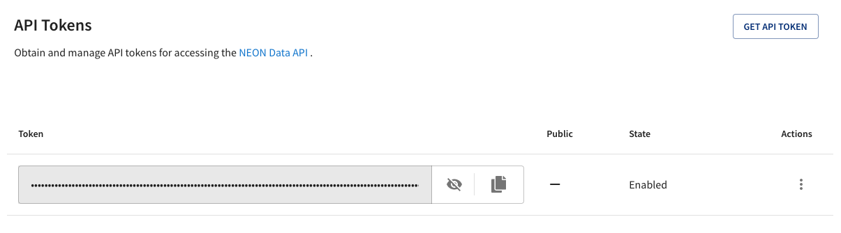
Once you have an account, you can create an API token for yourself. At the bottom of the My Account page, you should see this bar:

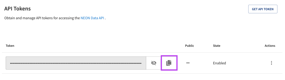
Click the ‘GET API TOKEN’ button. After a moment, you should see this:
Click on the Copy button to copy your API token to the clipboard:
Use API token in neonUtilities
In the next section, we’ll walk through saving your token somewhere secure but accessible to your code. But first let’s try out using the token the easy way, by using it as a simple text string.
NEON API tokens are very long, so it would be annoying to keep pasting the entire string into functions. Assign your token an object name:
R
NEON_TOKEN <- "PASTE YOUR TOKEN HERE"Now we’ll use the loadByProduct() function to download
data. Your API token is entered as the optional token input
parameter. For this example, we’ll download Plant foliar traits
(DP1.10026.001).
foliar <- loadByProduct(dpID="DP1.10026.001", site="all",
package="expanded", check.size=F,
token=NEON_TOKEN)Python
NEON_TOKEN = "PASTE YOUR TOKEN HERE"Now we’ll use the load_by_product() function to download
data. Your API token is entered as the optional token input
parameter. For this example, we’ll download Plant foliar traits
(DP1.10026.001).
foliar = nu.load_by_product(dpid="DP1.10026.001", site="all",
package="expanded", check_size=False,
token=NEON_TOKEN)You should now have data saved in the foliar object; the
API silently used your token. If you’ve downloaded data without a token
before, you may notice this is faster!
This format applies to all neonUtilities functions that
involve downloading data or otherwise accessing the API; you can use the
token input with all of them. For example, when downloading
remote sensing data:
Use token to download AOP data
R
chm <- byTileAOP(dpID="DP3.30015.001", site="WREF",
year=2017, check.size=F,
easting=c(571000,578000),
northing=c(5079000,5080000),
savepath=getwd(),
token=NEON_TOKEN)Python
chm = nu.by_tile_aop(dpid="DP3.30015.001", site="WREF",
year=2017, check_size=False,
easting=[571000,578000],
northing=[5079000,5080000],
savepath=os.getcwd(),
token=NEON_TOKEN)Token management for open code
Your API token is unique to your account, so don’t share it!
If you’re writing code that will be shared with colleagues or
available publicly, such as in a GitHub repository or supplemental
materials of a published paper, you can’t include the line of code above
where we assigned your token to NEON_TOKEN, since your
token is fully visible in the code there. Instead, you’ll need to save
your token locally on your computer, and pull it into your code without
displaying it. There are a few ways to do this, we’ll show two options
here.
Option 1: Save the token in a local file, and
source()(R) orimport(Python) that file at the start of every script. This is fairly simple but requires a line of code in every script.Option 2: Set the token as an environment variable and you can access it from any script. This is a little harder to set up initially, but once it’s done, it’s done globally, and it will work in every script you run.
Option 1: Save token in a local file
R
Open a new, empty R script (.R). Put a single line of code in the script:
NEON_TOKEN <- "PASTE YOUR TOKEN HERE"Save this file in a logical place on your machine, somewhere that
won’t be visible publicly. Here, let’s call the file
neon_token_source.R, and save it to the working directory.
Then, at the start of every script where you’re going to use the NEON
API, you would run this line of code:
source(paste0(wd, "/neon_token_source.R"))Now you can use token=NEON_TOKEN when you run
neonUtilities functions, and you can share your code
without accidentally sharing your token.
Python
Open a new, empty Python script (.py). Put a single line of code in the script:
NEON_TOKEN = "PASTE YOUR TOKEN HERE"Save this file in a logical place on your machine, somewhere that
won’t be visible publicly. Here, let’s call the file
neon_token_source.py, and save it to the working directory.
Then, at the start of every script where you’re going to use the NEON
API, you would run this line of code:
import neon_token_sourceNow you can use token=neon_token_source.NEON_TOKEN when
you run neonutilities functions, and you can share your
code without accidentally sharing your token.
Option 2: Set token as environment variable
R
To create a persistent environment variable in R, we use a
.Renviron file. Before creating a file, check which
directory R is using as your home directory:
# For Windows:
Sys.getenv("R_USER")
For Mac/Linux:
Sys.getenv("HOME")
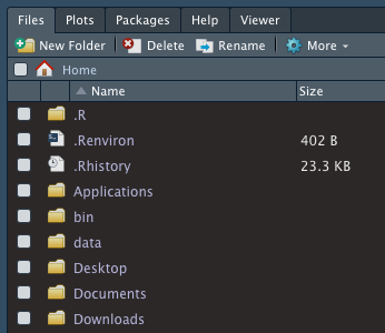
Check the home directory to see if you already have a
.Renviron file, using the file browse pane in
RStudio, or using another file browse method with hidden files
shown. Files that begin with . are hidden by default, but
RStudio recognizes files that begin with .R and displays
them.
If you already have a .Renviron file, open it and follow
the instructions below to add to it. If you don’t have one, create one
using File -> New File -> Text File in the RStudio menus.
Add one line to the text file. In this case, there are no quotes around the token value.
NEON_TOKEN=PASTE YOUR TOKEN HERESave the file as .Renviron, in the RStudio home
directory identified above. Double check the spelling, this will not
work if you have a typo. Re-start R to load the environment.
Once your token is assigned to an environment variable, use the
function Sys.getenv() to access it. For example, in
loadByProduct():
foliar <- loadByProduct(dpID="DP1.10026.001", site="all",
package="expanded", check.size=F,
token=Sys.getenv("NEON_TOKEN"))Python
To create a persistent environment variable in Python, the simplest
option is to use the dotenv module. You will still need to
load the variables in each script, but it provides a more flexible way
to manage enrionment variables.
pip install python-dotenvCreate a file named .env in the project folder. If
you’re using GitHub, make sure .env is in your
.gitignore to avoid syncing tokens to GitHub.
To add variables to the .env file:
import dotenv
dotenv.set_key(dotenv_path=".env",
key_to_set="NEON_TOKEN",
value_to_set="YOUR TOKEN HERE")
Use the command dotenv.load_dotenv() to load environment
variables to the session, then use os.environ.get() to
access particular variables. For example, in
load_by_product():
dotenv.load_dotenv()foliar = nu.load_by_product(dpid="DP1.10026.001", site="all",
package="expanded", check_size=False,
token=os.environ.get("NEON_TOKEN"))If dotenv.load_dotenv() returns False, the
variables did not load. Try
dotenv.load_dotenv(dotenv.find_dotenv(usecwd=True)).
Get Lesson Code
Understanding Releases and Provisional Data
Last Updated: Apr 2, 2026
What is a data release?
A NEON data Release is a fixed set of data that does not change over time. Each data product in a Release is associated with a unique Digital Object Identifier (DOI) that can be used for data citation. Since the data in a Release do not change, analyses performed on those data are traceable and reproducible.
NEON data are initially published under a Provisional status, meaning that data may be updated on an as-needed basis, without guarantee of reproducibility. Publishing Provisional data allows NEON to publish data rapidly while retaining the ability to make corrections or additions as they are identified.
After initial publication, a lag time occurs before the data are formally Released. During this lag time, extra quality control (QC) procedures, which are described in data product-specific documentation, may be performed. This lag time also ensures all data from laboratory analyses that complement existing field data are available before a data Release.
Although data within a Release do not change, NEON may discover errors or needed updates to data after the publication of a Release. For this reason, NEON generates a Release annually; each Release represents the best data available at the time of publication. Changes to data between Releases are documented on the web page for each Release and in the issue log for each data product.
Data citation
Each data product within a Release is associated with a DOI for reference and citation. DOI URLs will always resolve back to their corresponding data product Release’s landing webpage and are thus ideal for citing NEON data in publications and applications.
For more details about NEON data Releases, see the Data Product Revisions and Releases web page.
Objectives
After completing this activity, you will be able to:
- Download data from a specific NEON data Release
- Download Provisional NEON data
- Use appropriate citation information for both Released and Provisional data
Things You’ll Need To Complete This Tutorial
Most of this tutorial can be completed with nothing but an internet browser, without writing any code. You can learn about Releases and Provisional data and explore them on the Data Portal, and view figures from the data downloads.
To complete the full tutorial, including the coding sections, you will need a version of R (4.0 or higher) and, preferably, RStudio loaded on your computer. This code may work with earlier versions but it hasn't been tested.
Install R Packages
-
neonUtilities:
install.packages("neonUtilities")
Additional Resources
- NEON Data Portal
- NEON Code Hub
Set Up R Environment
First install and load the necessary packages.
# install packages. can skip this step if
# the packages are already installed
install.packages("neonUtilities")
# load packages
library(neonUtilities)
library(ggplot2)
# set working directory
# modify for your computer
setwd("~/data")
Find data of interest
We'll start with the Explore Data Products page on the NEON Data Portal, which has visual interfaces to allow you to select a particular Release, and show you which data are included in it.
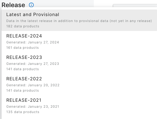
On the lefthand menu bar, the dropdown menu of Releases shows the available releases and the default display, which is the latest Release plus Provisional data.
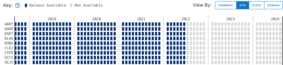
Stay on the default menu option for now. Navigate to quantum line PAR, DP1.00066.001. Expand the data availability chart by clicking on View By: SITE.
What you see will probably not look exactly like this, but similar. This is a screenshot from January 2024; more data and possibly more Releases may have been published by the time you follow this tutorial.
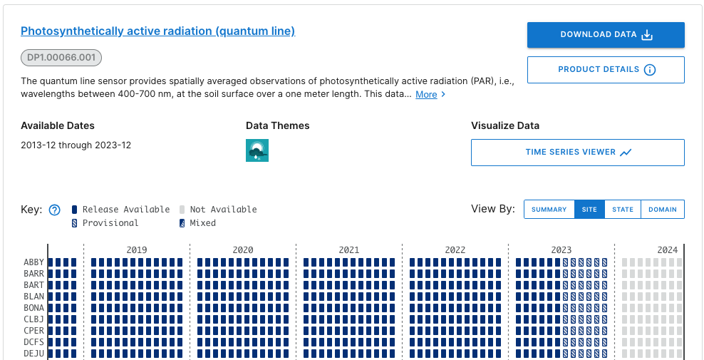
Here we can consult the key and see that data up to June 2023 are in a Release (solid boxes) and data collected since June 2023 are Provisional (hatched boxes). There are no 2024 data available yet (pale grey boxes).
Now click on the Product Details button to go to the DP1.00066.001 web page.
This page contains details and documentation about the data product, including citation information for publications using these data.
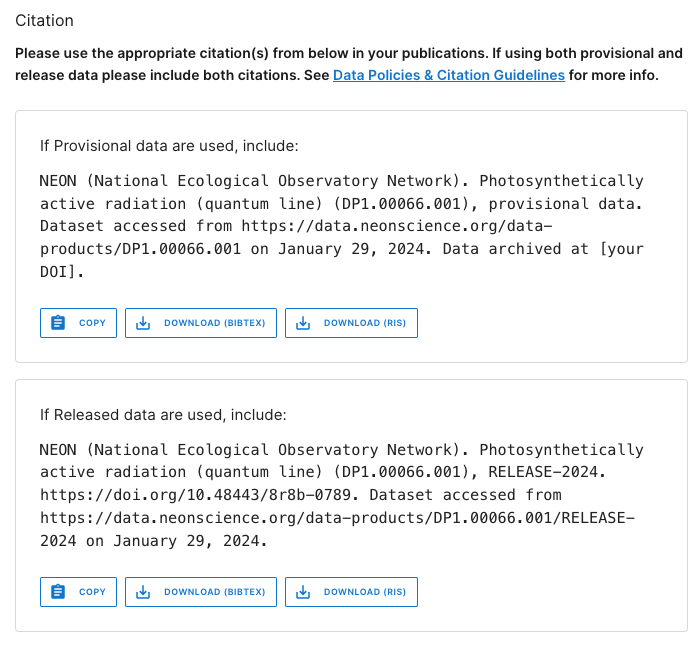
Note that the citation guidance is different for Provisional and Released data. The Release citation includes a direct link to a DOI. Since Provisional data are subject to change without notice, the data you download today may not exactly match data you download tomorrow. Because of this, the recommended workflow is to archive the version of Provisional data you used in your analyses, and provide a DOI to that archived version for citation. Guidance in doing this is available on the Publishing Research Outputs web page.
Downloading data
Latest and provisional
Go back to the main Explore Data Products page and click on Download Data. Select BARR (Utquiagvik) and BONA (Caribou Creek) for the year of 2023. Click Next.
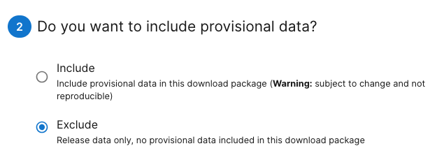
By default, the download options are set to access the latest Release and exclude Provisional data, even if they are available in the sites and dates you selected. To download Provisional data, select the radio button for Include in the interface.
Download by Release
But let's say you're not looking for the most recently updated data. You're replicating a colleague's analysis, and want to download the precise version of data they used. In that case, you need to download the Release they used.
Go back to the Explore Data Products page, and select the Release you need from the Release menu on the lefthand bar. For this example, let's use RELEASE-2023.
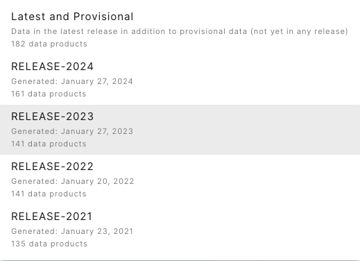
Now, in the data availability chart, we can see there are no hatched boxes, since we've selected only data that are in a Release. And data availability extends only through June 2022, the end date for sensor data in RELEASE-2023.
Downloading data using neonUtilities
NEON data can also be downloaded in R, using the neonUtilities package. If
you're not familiar with the neonUtilities package and how to use
it to access NEON data, we recommend you follow the Download and Explore NEON Data
tutorial as well as this one, for a more complete introduction.
Downloading the latest Release and Provisional
Let's download a full year of data for two sites, as we did on the Data Portal above. Here we'll download data from HEAL (Healy) and GUAN (Guanica), January 2023 - December 2023.
(Note: To see the code behavior below, if you are following this tutorial in 2025 or later, you may need to adjust the dates. In general, use the most recent full year of data.)
qpr <- loadByProduct(dpID="DP1.00066.001",
site=c("HEAL", "GUAN"),
startdate="2023-01",
enddate="2023-12",
check.size=F)
In the messages output as this function runs, you will see:
Provisional data were excluded from available files list. To download provisional data, use input parameter include.provisional=TRUE.
Just like on the Data Portal, you need to opt in to download Provisional data. We'll do that below. But first, let's take a look at the data we downloaded:
gg <- ggplot(qpr$PARQL_30min,
aes(endDateTime, linePARMean)) +
geom_line() +
facet_wrap(~siteID)
gg
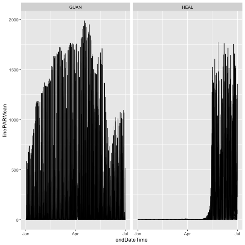
As we can see, the only data present from 2023 are from the first half of the year, the data included in RELEASE-2024. Provisional data from July 2023 onward were omitted.
Now let's download the Provisional data as well:
qpr <- loadByProduct(dpID="DP1.00066.001",
site=c("HEAL", "GUAN"),
startdate="2023-01",
enddate="2023-12",
include.provisional=T,
check.size=F)
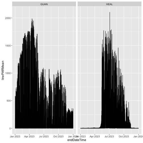
And now plot the full year of data:
gg <- ggplot(qpr$PARQL_30min,
aes(endDateTime, linePARMean)) +
geom_line() +
facet_wrap(~siteID)
gg
Downloading by Release
To download a specific Release, add the input parameter release=.
Let's download the data from collection year 2021 in RELEASE-2023.
qpr23 <- loadByProduct(dpID="DP1.00066.001",
site=c("HEAL", "GUAN"),
startdate="2021-01",
enddate="2021-12",
release="RELEASE-2023",
check.size=F)
What types of differences might there be in data from different Releases? Let's look at the same data set in RELEASE-2024.
qpr24 <- loadByProduct(dpID="DP1.00066.001",
site=c("HEAL", "GUAN"),
startdate="2021-01",
enddate="2021-12",
release="RELEASE-2024",
check.size=F)
Plot mean PAR from each release. This time we'll only use data from soil plot 001, to simplify the figure. We'll plot RELEASE-2023 in black and RELEASE-2024 in partially transparent blue, to see differences where they're overlaid.
gg <- ggplot(qpr23$PARQL_30min
[which(qpr23$PARQL_30min$horizontalPosition=="001"),],
aes(endDateTime, linePARMean)) +
geom_line() +
facet_wrap(~siteID) +
geom_line(data=qpr24$PARQL_30min
[which(qpr24$PARQL_30min$horizontalPosition=="001"),],
color="blue", alpha=0.3)
gg
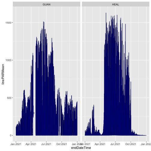
The blue and black lines are basically identical; the mean PAR data have not changed between the two releases. We can consult the issue log to see if there are any changes recorded for other variables in the data.
tail(qpr24$issueLog_00066)
## id parentIssueID issueDate resolvedDate dateRangeStart
## <int> <int> <char> <char> <char>
## 1: 45613 NA 2022-01-18T00:00:00Z 2022-01-01T00:00:00Z 2013-01-01T00:00:00Z
## 2: 60104 NA 2022-07-05T00:00:00Z 2022-10-19T00:00:00Z 2021-10-15T00:00:00Z
## 3: 66607 NA 2022-09-12T00:00:00Z 2022-10-31T00:00:00Z 2022-06-12T00:00:00Z
## 4: 78006 NA 2023-03-02T00:00:00Z 2023-11-03T00:00:00Z 2023-03-02T00:00:00Z
## 5: 78310 NA 2023-03-16T00:00:00Z 2023-03-31T00:00:00Z 2014-02-18T00:00:00Z
## 6: 85004 NA 2024-01-04T00:00:00Z 2024-01-04T00:00:00Z 2013-12-01T00:00:00Z
## dateRangeEnd locationAffected
## <char> <char>
## 1: 2021-10-01T00:00:00Z All
## 2: 2022-10-19T00:00:00Z WREF soil plot 3 (HOR.VER: 003.000)
## 3: 2022-10-31T00:00:00Z YELL
## 4: 2023-11-03T00:00:00Z All
## 5: 2023-03-01T00:00:00Z All CPER soil plots (HOR: 001, 002, 003, 004, and 005)
## 6: 2023-12-31T00:00:00Z All terrestrial sites
## issue
## <char>
## 1: Data were reprocessed to incorporate minor and/or isolated corrections to quality control thresholds, sensor installation periods, geolocation data, and manual quality flags.
## 2: Sensor malfunction indicated by positive nighttime radiation
## 3: Severe flooding destroyed several roads into Yellowstone National Park in June 2022, making the YELL and BLDE sites inaccessible to NEON staff. Preventive and corrective maintenance were not able to be performed, nor was the annual exchange of sensors for calibration and validation. While automated quality control routines are likely to detect and flag most issues, users are advised to review data carefully.
## 4: Photosynthetically active radiation (quantum line) measurement height (zOffset) incorrectly shown as 0 m in the sensor positions file in the download package. The actual measurement height is 3+ cm above the soil surface.
## 5: Two different soil plot reference corner records were created for each CPER soil plot, which resulted in two partially different sets of sensor location data being reported in the sensor_positions file. Affected variables were referenceLatitude, referenceLongitude, referenceElevation, eastOffset, northOffset, xAzimuth, and yAzimuth. Other sensor location metadata, including sensor height/depth (zOffset), were unaffected but were still reported twice for each sensor.
## 6: Photosynthetically active radiation (quantum line) (DP1.00066.001) has been reprocessed using NEON’s new instrument processing pipeline. Computation of skewness and kurtosis statistics has been updated in the new pipeline. Previously, these statistics were computed with the Apache Commons Mathematics Library, version 3.6.1, which uses special unbiased formulations and not those described in the Algorithm Theoretical Basis Document (ATBD), which cites the standard formulations. Differences in data values between previous and reprocessed data for the skewness statistic are typically < 1% for 30-min averages and < 10% for 1-min averages. Differences for the kurtosis statistic are much larger, as the previous version reported excess kurtosis which subtracts a value of three so that a normal distribution is equal to zero. Thus, new values for kurtosis are typically greater by 3 ± 1% for 30-min averages and 3 ± 10% for 1-min averages.
## resolution
## <char>
## 1: Reprocessed provisional data are available now. Reprocessed data previously included in RELEASE-2021 will become available when RELEASE-2022 is issued.
## 2: Data flagged and sensor cable replaced.
## 3: Normal operations resumed on October 31, 2022, when the National Park Service opened a newly constructed road from Gardiner, MT to Mammoth, WY with minimal restrictions. For more details about data impacts, see Data Notification https://www.neonscience.org/impact/observatory-blog/data-impacts-neons-yellowstone-sites-yell-blde-due-catastrophic-flooding-0
## 4: Measurement heights have been added and data republication has been requested, which should be completed within a few weeks. Heights will be available from July 2022 onwards once data republication is complete and will be available for all data once RELEASE-2024 data are published (expected January 2024). The issue will persist in RELEASE-2023 data and prior data releases.
## 5: The erroneous reference corner record was deleted and data were scheduled for republication. This issue will persist in data from June 2022 and earlier until the RELEASE-2024 data is published (approximately January 2024). It will also persist in RELEASE-2023 and earlier data releases.
## 6: All provisional data have been updated, and data for all time and all sites will be updated in RELEASE-2024 (expected to be issued in late January, 2024).
The final issue noted in the table was reported and resolved in January 2024. It tells us that the data were reprocessed for the 2024 Release, and the algorithms for the skewness and kurtosis statistics were updated. Let's take a look at the kurtosis statistics from the two Releases.
gg <- ggplot(qpr23$PARQL_30min
[which(qpr23$PARQL_30min$horizontalPosition=="001"),],
aes(endDateTime, linePARKurtosis)) +
geom_line() +
facet_wrap(~siteID) +
geom_line(data=qpr24$PARQL_30min
[which(qpr24$PARQL_30min$horizontalPosition=="001"),],
color="blue", alpha=0.3)
gg
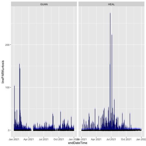
Here, we can see the kurtosis values have shifted slightly higher in RELEASE-2024, relative to their values in RELEASE-2023. This is a metric of the distribution of PAR observations within the averaging interval; if this aspect of variability is important for your analysis, you would now be able to incorporate these improved estimates into your work.
Data citation
We saw above that citation information is available on the data product detail
pages on the Data Portal. The neonUtilities package functions also provide
citations in BibTeX.
Provisional:
writeLines(qpr$citation_00066_PROVISIONAL)
## @misc{DP1.00066.001/provisional,
## doi = {},
## url = {https://data.neonscience.org/data-products/DP1.00066.001},
## author = {{National Ecological Observatory Network (NEON)}},
## language = {en},
## title = {Photosynthetically active radiation (quantum line) (DP1.00066.001)},
## publisher = {National Ecological Observatory Network (NEON)},
## year = {2024}
## }
RELEASE-2024:
writeLines(qpr$`citation_00066_RELEASE-2024`)
## @misc{https://doi.org/10.48443/8r8b-0789,
## doi = {10.48443/8R8B-0789},
## url = {https://data.neonscience.org/data-products/DP1.00066.001/RELEASE-2024},
## author = {{National Ecological Observatory Network (NEON)}},
## keywords = {solar radiation, soil surface radiation, photosynthetically active radiation (PAR), photosynthetic photon flux density (PPFD), quantum line sensor},
## language = {en},
## title = {Photosynthetically active radiation (quantum line) (DP1.00066.001)},
## publisher = {National Ecological Observatory Network (NEON)},
## year = {2024},
## copyright = {Creative Commons Zero v1.0 Universal}
## }
These can be adapted as needed for other formatting conventions.
Data management
Within the neonUtilities package, some functions download data, some
perform data wrangling on data you've already downloaded, and some do
both. Different approaches are practical for Released and Provisional
data.
Since data in a Release never change, there's no need to download a Release multiple times. On the other hand, if you're working with Provisional data, you may want to re-download each time you work on an analysis, to ensure you're always working with the most up-to-date data.
The neonUtilities cheat sheet includes an overview
of the operations carried out by each function, for reference.
Here, we'll outline some suggested workflows for data management, organized by NEON measurement system.
Sensor or observational (IS/OS)
Most people working with NEON's tabular data (OS and IS) use the
loadByProduct() function to download and stack data files. It
downloads data from the NEON API every time you run it. When
working with data in a Release, it can be convenient to save the
downloaded data as an R object and re-load it the next time you
work on your analysis, rather than downloading again.
tick <- loadByProduct(dpID="DP1.10093.001",
site=c("GUAN"),
release="RELEASE-2024",
check.size=F)
saveRDS(tick, paste0(getwd(), "/NEON_tick_data.rds"))
And the next time you start work:
tick <- readRDS(paste0(getwd(), "/NEON_tick_data.rds"))
When working with Provisional data, you can run
loadByProduct() every time to get the most recent data, but
be sure to save and archive the final version you use in a
publication, for citation and reproducibility. Guidelines for
archiving a dataset can be found on the
Publishing Research Outputs webpage.
Eddy covariance or atmospheric isotopes (SAE)
Because SAE files are so large, stackEddy() is designed to extract
the desired variables from locally stored files, and it works the
same way on files downloaded from the Data Portal or by
zipsByProduct(). You can download once, using your preferred method,
and then use stackEddy() every time you need to access any of the
file contents.
zipsByProduct(dpID="DP4.00200.001",
site=c("TEAK"),
startdate="2023-05",
enddate="2023-06",
release="RELEASE-2024",
savepath=getwd(),
check.size=F)
flux <- stackEddy(paste0(getwd(), "/filesToStack00200"),
level="dp04")
The next time you need to work with these data, you can skip the
zipsByProduct() line and go straight to stackEddy(). And if you
come back later and decide you want to work with the isotope data
instead of the flux data, still no need to re-download:
iso <- stackEddy(paste0(getwd(), "/filesToStack00200"),
level="dp01", var="isoCo2", avg=6)
If you're working with Provisional SAE data, you may be thinking you'll need to re-download regularly. But SAE data are rarely re-processed outside of the annual release schedule, due to the large computational demands of SAE processing. Each month, you can download newly published Provisional data that were collected the previous month, but you won't need to re-download older months.
Remote sensing (AOP)
Data Releases are handled a bit differently for AOP than the other data systems. Due to the very large volume of data, past Releases of AOP data are not available for download. Only the most recent Release and Provisional data can be downloaded at any given time.
DOIs for past Releases of AOP data remain available, and can be used to cite the data in perpetuity. Their DOI status is set to "tombstone", the term used to denote a dataset that is citable but no longer accessible.
See the Large Data Packages section on the Publishing Research Outputs page for suggestions about archiving large datasets.
Get Lesson Code
Understanding AOP Data Releases and Best Practices for AOP Data Management
Last Updated: Apr 2, 2026
What is a NEON Data Release?
A NEON Data Release is a fixed set of data that does not change over time. Each data product in a Release is associated with a unique Digital Object Identifier (DOI) that can be used for data citation. Because the data in a Release do not change, analyses performed on those data are traceable and reproducible.
NEON data are initially published under a Provisional status, meaning that data may be updated on an as-needed basis, without guarantee of reproducibility. Publishing Provisional data allows NEON to publish data rapidly while retaining the ability to make corrections or additions as the need is identified. Most of the time, unless issues are discovered in the Provisional data, the Provisional data will become Released - so Provisional data are still valid to use. If any issues are identified, they will be included in the data product issue logs.
For more details about NEON Data Releases, see the Understanding Releases and Provisional Data tutorial and the Data Product Revisions and Releases web page.
How are AOP Releases different than the other NEON subsystems (IS/OS)?
Unlike NEON's other systems (Instrumented/IS and Observational/OS), AOP (Remote Sensing) does not preserve historical versions of data. Most AOP data products are high volume; thus it is expensive to store and make openly and freely available more than the most recent version. Therefore, NEON's annual releases for AOP data products are only available for the current release year – from the date of release to approximately 11 months later when the AOP team begins preparing for the next year’s release. For example, Release-2023 versions of AOP data products were available from January 27, 2023 until December 20, 2023.
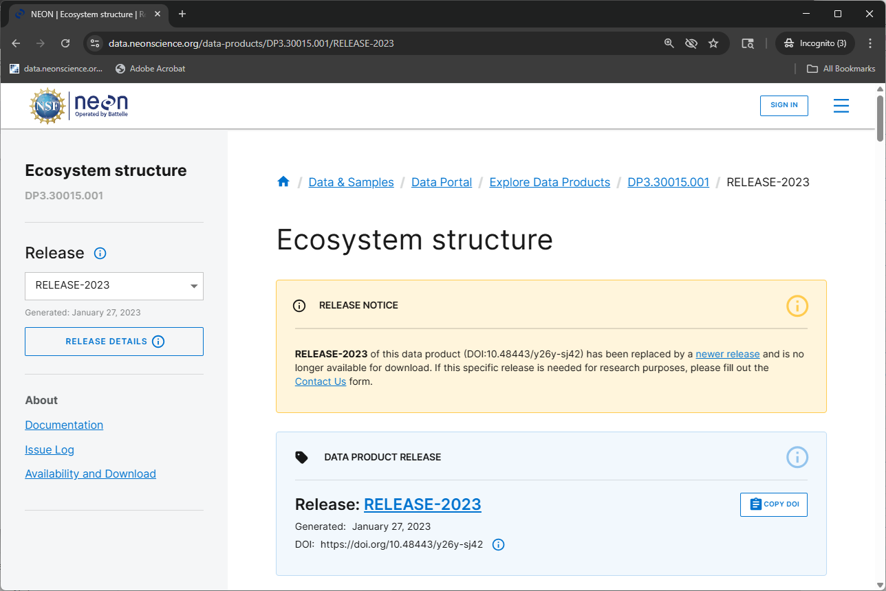
DOIs for AOP data products for a given RELEASE will be tombstoned prior to each subsequent Release. These tombstoned data can be thought of as being "out of print": the DOI for each data product release is still valid, but the version of the data that the DOI referred to is no longer available for download. A DOI that has been tombstoned will resolve to the data product release's webpage which explains that the released version of the product is no longer available for download (e.g. Ecosystem structure RELEASE-2023, also shown in the figure below).
Prior to each annual NEON Release, AOP scientists review the existing data and reprocess data if any issues are identified. Then they begin an approximately month-long transition period of replacing older files with newer ones. During this period, the current data release tag may no longer point to the same exact files for certain AOP data products that are undergoing updates. Although the data portal or API may indicate availability of a data product at specific sites for specific months, some files may be unavailable for few days (or longer) before being replaced by updated versions.
NEON will publish a Data Notification indicating when AOP is transitioning between one Release and the next (e.g., AOP Data Availability Notification – Release 2024). We suggest holding off on downloading AOP data during this interim period if it is not urgent, or submitting an inquiry through the NEON Contact Us Form to obtain information about the status of the data products, sites, and years that you are interested in.
How can I tell if the AOP data I've downloaded is up to date?
There are a few ways to check if and what AOP data have been updated since you last downloaded the data, both on the website, and programmatically using functionality built into the AOP download functions. On the website, you can check the Issue Log tables on each data product page and also see the Issue resolutions, and you can also check the Release pages for a complete summary of what has been changed between the past release and the current one; for example Release 2025. This tutorial will demonstrate some of the programmatic options to check if published AOP data has been modified compared to your local version.
Objectives
After completing this activity, you will be able to:
- Find available Released and Provisional AOP data for a given site and data product
- Understand options for downloading AOP data
- Display citation information for both Released and Provisional data
- Learn about available tools to reduce large data downloads
- Understand some basic best practices for working with large volumes of AOP data
Things You’ll Need To Complete This Tutorial
To complete this tutorial, you will need a version of Python (3.9 or higher), the latest Python neonutilities package (1.2 or higher) and, preferably, Jupyter Notebooks or Spyder installed on your computer. Much of the lesson can also be carried out in R using the R neonUtilities package; however some of the functionality that is demonstrated is currently only available in Python.
Additional Resources
Import Required Packages
For this tutorial, we will mainly be exploring the functions imported below in the neonutilities package that allow us to explore availability of and download AOP data.
import csv
import os
from neonutilities import by_file_aop, list_available_dates, get_citation
First, we can use some the list_available_dates function to find available data. This will show us the data that is available both provisionally and as part of the latest release. First, run help(list_available_dates) to see the required inputs of this function.
help(list_available_dates)
Help on function list_available_dates in module neonutilities.aop_download:
list_available_dates(dpid, site)
list_available_dates displays the available releases and dates for a given product and site
--------
Inputs:
dpid: the data product code (eg. 'DP3.30015.001' - CHM)
site: the 4-digit NEON site code (eg. 'JORN')
--------
Returns:
prints the Release Tag (or PROVISIONAL) and the corresponding available dates (YYYY-MM) for each tag
--------
Usage:
--------
>>> list_available_dates('DP3.30015.001','JORN')
RELEASE-2025 Available Dates: 2017-08, 2018-08, 2019-08, 2021-08, 2022-09
>>> list_available_dates('DP3.30015.001','HOPB')
PROVISIONAL Available Dates: 2024-09
RELEASE-2025 Available Dates: 2016-08, 2017-08, 2019-08, 2022-08
>>> list_available_dates('DP1.10098.001','HOPB')
ValueError: There are no data available for the data product DP1.10098.001 at the site HOPB.
The required inputs for this function are the data product id (dpid) and the site code (site). Let's try this out for the Canopy Height Model (Ecosystem Structure) data product at the McRae Creek site in Oregon (MCRA), to start. The CHM data product has the code DP3.30015.001.
list_available_dates('DP3.30015.001','MCRA')
PROVISIONAL Available Dates: 2025-08
RELEASE-2025 Available Dates: 2018-07, 2021-07, 2022-07, 2023-07
We can see that as of Dec 2025, CHM data at MCRA are available provisionally in 2025, and as part of RELEASE-2025 for the years 2018, 2021, 2022, and 2023. MCRA is a non-collocated aquatic site and is collected on an opportunistic basis, so it has been flown a little less frequently than the terrestrial or collocated aquatic sites.
We can download the CHM data from the site MCRA collected in 2023 and 2025 using the neonutilities function by_file_aop. Note that by_file_aop downloads all available data for a given data product, while by_tile_aop downloads only data that intersect provided UTM coordinates (easting and northing). For the purposes of this tutorial, we will stick to using by_file_aop, but note that you could use by_tile_aop similarly, provided you know which tiles you want to download. First, take a quick look at the function documentation using help.
help(by_file_aop)
Help on function by_file_aop in module neonutilities.aop_download:
by_file_aop(dpid, site, year, include_provisional=False, check_size=True, savepath=None, chunk_size=1024, token=None, verbose=False, skip_if_exists=False, overwrite='prompt')
This function queries the NEON API for AOP data by site, year, and product, and downloads all
files found, preserving the original folder structure. It downloads files serially to
avoid API rate-limit overload, which may take a long time.
Parameters
--------
dpid: str
The identifier of the NEON data product to pull, in the form DPL.PRNUM.REV, e.g. DP3.30001.001.
site: str
The four-letter code of a single NEON site, e.g. 'CLBJ'.
year: str or int
The four-digit year of data collection.
include_provisional: bool, optional
Should provisional data be downloaded? Defaults to False. See
https://www.neonscience.org/data-samples/data-management/data-revisions-releases
for details on the difference between provisional and released data.
check_size: bool, optional
Should the user approve the total file size before downloading? Defaults to True.
If you have sufficient storage space on your local drive, when working
in batch mode, or other non-interactive workflow, use check_size=False.
savepath: str, optional
The file path to download to. Defaults to None, in which case the working directory is used.
chunk_size: integer, optional
Size in bytes of chunk for chunked download. Defaults to 1024.
token: str, optional
User-specific API token from data.neonscience.org user account. Defaults to None.
See https://data.neonscience.org/data-api/rate-limiting/ for details about API
rate limits and user tokens.
verbose: bool, optional
If set to True, the function will print more detailed information about the download process.
skip_if_exists: bool, optional
If set to True, the function will skip downloading files that already exist in the
savepath and are valid (local checksums match the checksums of the published file).
Defaults to False. If any local file checksums don't match those of files published
on the NEON Data Portal, the user will be prompted to skip these files or overwrite
the existing files with the new ones (see overwrite input).
overwrite: str, optional
Must be one of:
'yes' - overwrite mismatched files without prompting,
'no' - don't overwrite mismatched files (skip them, no prompt),
'prompt' - prompt the user (y/n) to overwrite mismatched files after displaying them (default).
If skip_if_exists is False, this parameter is ignored, and any existing files in
the savepath will be overwritten according to the function's default behavior.
Returns
--------
None; data are downloaded to the directory specified (savepath) or the current working directory.
If data already exist in the expected path, they will be overwritten by default. To check for
existing files before downloading, set skip_if_exists=True along with an overwrite option (y/n/prompt).
Examples
--------
>>> by_file_aop(dpid="DP3.30015.001",
site="MCRA",
year="2021",
savepath="./test_download",
skip_if_exists=True)
# This downloads the 2021 Canopy Height Model data from McRae Creek to the './test_download' directory.
# If any files already exist in the savepath, they will be checked and skipped if they are valid.
# The user will be prompted to ovewrite or skip downloading any existing files that do not match
# the latest published data on the NEON Data Portal.
Notes
--------
This function creates a folder named by the Data Product ID (DPID; e.g. DP3.30015.001) in the
'savepath' directory, containing all AOP files meeting the query criteria. If 'savepath' is
not provided, data are downloaded to the working directory, in a folder named by the DPID.
The required inputs for this function are the data product id (dpid), site id (site) and year (year). Note that there are a number of additional optional inputs, which we will explain more in detail. Some ones that we recommend paying attention to are:
-
token: Your API token from your NEON user account (on data.neonscience.org). Currently defaults to None, but we highly encourage using a token when downloading NEON data. See Using an API Token when Accessing NEON Data with neonUtilities for more details on the benefits of tokens and how to use them. -
include_provisional: setting this toTrueis the only way you can download provisional data. If you've used thelist_available_datesfunction and you want to download data from a year where it is only available provisionally, you must set this option to True in order to download any data. You will see a warning if no data are found. We will show this in the example below. -
savepath: this is the path where data will be downloaded. We recommend setting this to somewhere close to the root folder to avoid very long paths for AOP data. Windows systems can have path length limitations (unless you change them) and if the path is too long you may see a warning or error.
In the most recent version of Python neonutilities (1.2.0, released in October 2025), there are two new optional inputs to the by_file_aop and by_tile_aop functions: skip_if_exists and overwrite. We will go over these options in more detail towards the end of this tutorial. For now, just know that these options provide functionality to avoid re-downloading identical data.
Set the data directory, where data will be downloaded. Make sure this is a path that works on your system and has sufficient space for downloading data.
data_dir = r'C:\NEON_Data'
by_file_aop(dpid='DP3.30015.001',
site='MCRA',
year='2025',
savepath=data_dir)
Provisional NEON data are not included. To download provisional data, use input parameter include_provisional=True.
No NEON data files found. Available data may all be provisional. To download provisional data, use input parameter include_provisional=True.
Now let's set include_provisional=True to see what happens. Select "y" when prompted to download the data (first ensuring you have enough space).
by_file_aop(dpid='DP3.30015.001',
site='MCRA',
year='2025',
savepath=data_dir,
include_provisional=True)
Provisional NEON data are included. To exclude provisional data, use input parameter include_provisional=False.
Continuing will download 32 NEON data files totaling approximately 342.5 MB. Do you want to proceed? (y/n) y
Downloading 32 NEON data files totaling approximately 342.5 MB
100%|██████████████████████████████████████████████████████████████████████████████████| 32/32 [00:42<00:00, 1.32s/it]
You can also optionally set check_size=False if you don't want to be prompted to type yes or no (y/n) after the data volume is displayed. If this is your first time downloading data, we recommend keeping the default setting so you can make sure you have enough space on your computer before downloading.
Ok, simple enough! Let's take a look at the data we have downloaded. We'll write a couple of functions to let us see the folders and some of the files that have been downloaded. Feel free to explore the directory in File Explorer on your own as well.
def get_folders_with_files(path):
"""
Returns a list of folders within the given path that contain files,
excluding folders that only contain subfolders or are empty.
Args:
path (str): The path to the directory to search.
Returns:
list: A list of full paths to folders containing files.
"""
folders_with_files = []
for root, dirs, files in os.walk(path):
# Check if the current 'root' directory contains any files
if files:
folders_with_files.append(root)
return folders_with_files
def display_files_in_subdirectories(path):
"""
Displays files within a given directory and its subdirectories.
Only the first 5 files are shown in each directory if more are present.
Args:
path (str): The path to the root directory to start scanning from.
"""
# if not os.path.isdir(path):
# print(f"Error: '{path}' is not a valid directory.")
# return
for dirpath, dirnames, filenames in os.walk(path):
if filenames:
print(f"\nDirectory: {dirpath}")
# Sort filenames for consistent output, then take the first 5
sorted_filenames = sorted(filenames)
files_to_display = sorted_filenames[:5]
for file in files_to_display:
print(f" - {file}")
if len(sorted_filenames) > 5:
print(f" ... ({len(sorted_filenames) - 5} more files not shown)")
Use these functions to see what we've downloaded:
get_folders_with_files(data_dir)
['C:\\NEON_Data\\DP3.30015.001',
'C:\\NEON_Data\\DP3.30015.001\\neon-aop-provisional-products\\2025\\FullSite\\D16\\2025_MCRA_5\\L3\\DiscreteLidar\\CanopyHeightModelGtif',
'C:\\NEON_Data\\DP3.30015.001\\neon-aop-provisional-products\\2025\\FullSite\\D16\\2025_MCRA_5\\Metadata\\DiscreteLidar\\Reports',
'C:\\NEON_Data\\DP3.30015.001\\neon-aop-provisional-products\\2025\\FullSite\\D16\\2025_MCRA_5\\Metadata\\DiscreteLidar\\TileBoundary',
'C:\\NEON_Data\\DP3.30015.001\\neon-publication\\NEON.DOM.SITE.DP3.30015.001\\MCRA\\20250801T000000--20250901T000000\\basic']
display_files_in_subdirectories(data_dir)
Directory: C:\NEON_Data\DP3.30015.001
- citation_DP3.30015.001_PROVISIONAL.txt
- issueLog_DP3.30015.001.csv
Directory: C:\NEON_Data\DP3.30015.001\neon-aop-provisional-products\2025\FullSite\D16\2025_MCRA_5\L3\DiscreteLidar\CanopyHeightModelGtif
- NEON_D16_MCRA_DP3_565000_4900000_CHM.tif
- NEON_D16_MCRA_DP3_565000_4901000_CHM.tif
- NEON_D16_MCRA_DP3_565000_4902000_CHM.tif
- NEON_D16_MCRA_DP3_565000_4903000_CHM.tif
- NEON_D16_MCRA_DP3_565000_4904000_CHM.tif
... (22 more files not shown)
Directory: C:\NEON_Data\DP3.30015.001\neon-aop-provisional-products\2025\FullSite\D16\2025_MCRA_5\Metadata\DiscreteLidar\Reports
- 2025080216_P3C1_SBET_QAQC.pdf
- 2025_MCRA_5_L1_discrete_lidar_qa.html
- 2025_MCRA_5_L3_discrete_lidar_qa.html
Directory: C:\NEON_Data\DP3.30015.001\neon-aop-provisional-products\2025\FullSite\D16\2025_MCRA_5\Metadata\DiscreteLidar\TileBoundary
- 2025_MCRA_5_TileBoundary.zip
Directory: C:\NEON_Data\DP3.30015.001\neon-publication\NEON.DOM.SITE.DP3.30015.001\MCRA\20250801T000000--20250901T000000\basic
- NEON.D16.MCRA.DP3.30015.001.readme.20250926T050145Z.txt
We can see that we've downloaded some files in subfolders under the C:\NEON_Data\DP3.30015.001 folder. The provisional data are stored in a provisional bucket (or cloud storage path) called neon-aop-provisional-products and the full path of the data as it is stored on cloud storage is preserved in order to maintain organization. This is helpful if you are working with multiple data products, sites, and/or years of data. Note that there is an L3\DiscreteLidar\CanopyHeightModelGtiffolder - this contains the Level 3 (L3) geotiff files (or .tif tiles), and there is also a Metadata\DiscreteLidar folder, which contains the subfolders called Reports and TileBoundary. The reports are informational documents (in pdf or html format) summarizing the processing parameters and useful quality information. The TileBoundary folder contains shapefiles and kml files that provide useful information about the extent of the data. Please explore the data more on your own!
Before continuing, let's take a quick look at the files citation_DP3.30015.001_PROVISIONAL.txt and issueLog_DP3.30015.001.csv that were downloaded in the C:\NEON_Data\DP3.30015.001 folder.
with open(r'C:\NEON_Data\DP3.30015.001\citation_DP3.30015.001_PROVISIONAL.txt', 'r', newline='') as file:
reader = csv.reader(file)
for row in reader:
print(row[0])
@misc{DP3.30015.001/provisional
doi = {}
url = {https://data.neonscience.org/data-products/DP3.30015.001}
author = {{National Ecological Observatory Network (NEON)}}
language = {en}
title = {Ecosystem structure (DP3.30015.001)}
publisher = {National Ecological Observatory Network (NEON)}
year = {2025}
}
Note that there is no DOI since the data are provisional.
We can also get the citation information from the neonutilities get_citation function as follows:
mcra_chm_provisional_citation = get_citation('DP3.30015.001','PROVISIONAL')
mcra_chm_provisional_citation
'@misc{DP3.30015.001/provisional,\n doi = {},\n url = {https://data.neonscience.org/data-products/DP3.30015.001},\n author = {{National Ecological Observatory Network (NEON)}},\n language = {en},\n title = {Ecosystem structure (DP3.30015.001)},\n publisher = {National Ecological Observatory Network (NEON)},\n year = {2025}\n}'
We can format this a little more nicely as follows:
mcra_chm_provisional_citation.split('\n')
['@misc{DP3.30015.001/provisional,',
' doi = {},',
' url = {https://data.neonscience.org/data-products/DP3.30015.001},',
' author = {{National Ecological Observatory Network (NEON)}},',
' language = {en},',
' title = {Ecosystem structure (DP3.30015.001)},',
' publisher = {National Ecological Observatory Network (NEON)},',
' year = {2025}',
'}']
Let's also download data that has been released. For this example, we'll download the CHM data from 2023. In this case, as we saw at the start, the data have been released as part of RELEASE-2025, so we do not need to set include_provisional=True (although it won't hurt).
We can re-run the get_folders_with_files function to see the new data that has been downloaded. Type "y" for yes when prompted.
by_file_aop(dpid='DP3.30015.001',
site='MCRA',
year='2023',
savepath=data_dir)
Continuing will download 124 NEON data files totaling approximately 94.3 MB. Do you want to proceed? (y/n) y
Downloading 124 NEON data files totaling approximately 94.3 MB
100%|████████████████████████████████████████████████████████████████████████████████| 124/124 [00:47<00:00, 2.62it/s]
get_folders_with_files(data_dir)
['C:\\NEON_Data\\DP3.30015.001',
'C:\\NEON_Data\\DP3.30015.001\\neon-aop-products\\2023\\FullSite\\D16\\2023_MCRA_4\\L3\\DiscreteLidar\\CanopyHeightModelGtif',
'C:\\NEON_Data\\DP3.30015.001\\neon-aop-products\\2023\\FullSite\\D16\\2023_MCRA_4\\Metadata\\DiscreteLidar\\Reports',
'C:\\NEON_Data\\DP3.30015.001\\neon-aop-products\\2023\\FullSite\\D16\\2023_MCRA_4\\Metadata\\DiscreteLidar\\TileBoundary\\kmls',
'C:\\NEON_Data\\DP3.30015.001\\neon-aop-products\\2023\\FullSite\\D16\\2023_MCRA_4\\Metadata\\DiscreteLidar\\TileBoundary\\shps',
'C:\\NEON_Data\\DP3.30015.001\\neon-aop-provisional-products\\2025\\FullSite\\D16\\2025_MCRA_5\\L3\\DiscreteLidar\\CanopyHeightModelGtif',
'C:\\NEON_Data\\DP3.30015.001\\neon-aop-provisional-products\\2025\\FullSite\\D16\\2025_MCRA_5\\Metadata\\DiscreteLidar\\Reports',
'C:\\NEON_Data\\DP3.30015.001\\neon-aop-provisional-products\\2025\\FullSite\\D16\\2025_MCRA_5\\Metadata\\DiscreteLidar\\TileBoundary',
'C:\\NEON_Data\\DP3.30015.001\\neon-publication\\NEON.DOM.SITE.DP3.30015.001\\MCRA\\20250801T000000--20250901T000000\\basic',
'C:\\NEON_Data\\DP3.30015.001\\neon-publication\\release\\tag\\RELEASE-2025\\NEON.DOM.SITE.DP3.30015.001\\MCRA\\20230701T000000--20230801T000000\\basic']
Now, in addition to the data in the neon-aop-provisional-products folder, we have new data in a neon-aop-products folder. This is important to pay attention to, especially if you plan to re-download data - once data have gone through quality checks and are released, they will be moved to the neon-aop-products folder. Let's take a look at the files, only in this neon-aop-products folder.
display_files_in_subdirectories(os.path.join(data_dir,'DP3.30015.001','neon-aop-products'))
Directory: C:\NEON_Data\DP3.30015.001\neon-aop-products\2023\FullSite\D16\2023_MCRA_4\L3\DiscreteLidar\CanopyHeightModelGtif
- NEON_D16_MCRA_DP3_565000_4900000_CHM.tif
- NEON_D16_MCRA_DP3_565000_4901000_CHM.tif
- NEON_D16_MCRA_DP3_565000_4902000_CHM.tif
- NEON_D16_MCRA_DP3_565000_4903000_CHM.tif
- NEON_D16_MCRA_DP3_566000_4900000_CHM.tif
... (15 more files not shown)
Directory: C:\NEON_Data\DP3.30015.001\neon-aop-products\2023\FullSite\D16\2023_MCRA_4\Metadata\DiscreteLidar\Reports
- 2023070115_P1C1_SBET_QAQC.pdf
- 2023_MCRA_4_L1_discrete_lidar_processing.pdf
- 2023_MCRA_4_L3_discrete_lidar_processing.pdf
Directory: C:\NEON_Data\DP3.30015.001\neon-aop-products\2023\FullSite\D16\2023_MCRA_4\Metadata\DiscreteLidar\TileBoundary\kmls
- NEON_D16_MCRA_DPQA_565000_4900000_boundary.kml
- NEON_D16_MCRA_DPQA_565000_4901000_boundary.kml
- NEON_D16_MCRA_DPQA_565000_4902000_boundary.kml
- NEON_D16_MCRA_DPQA_565000_4903000_boundary.kml
- NEON_D16_MCRA_DPQA_566000_4900000_boundary.kml
... (15 more files not shown)
Directory: C:\NEON_Data\DP3.30015.001\neon-aop-products\2023\FullSite\D16\2023_MCRA_4\Metadata\DiscreteLidar\TileBoundary\shps
- NEON_D16_MCRA_DPQA_565000_4900000_boundary.dbf
- NEON_D16_MCRA_DPQA_565000_4900000_boundary.prj
- NEON_D16_MCRA_DPQA_565000_4900000_boundary.shp
- NEON_D16_MCRA_DPQA_565000_4900000_boundary.shx
- NEON_D16_MCRA_DPQA_565000_4901000_boundary.dbf
... (75 more files not shown)
We can see that the contents of the CHM geotiff files and Metadata reports are similar to what we saw in the provisional bucket. In the TileBoundary folder, there are both kmls and shapefiles (.shp, .shx, .dbf, .prj). Note that in RELEASE-2026 all of the Metadata files will be consolidated into a single merged kml and shapefile with labels showing all of the individual tiles. This will greatly reduce the number of files that are downloaded. Stay tuned for this update in late January or early Februrary 2026!
AOP Data Management Considerations
Avoiding Downloading Data That You've Already Downloaded
For this tutorial, we chose to demonstrate data downloads for a small site, and a relatively small AOP data product (comprised of single-band geotiff files). However, some of the other AOP datasets such as the surface reflectance data (426 bands) and the L1 discrete and waveform lidar data can be very large in size, especially for the typical 10 x 10 km terrestrial sites (or in some cases, larger)! If you are working with geotiff data for multiple years and sites, the data volume can also quickly add up. So what if you've already downloaded some AOP data and only want to pull data that has been updated, or make sure your data is up-to-date with the latest release?
The latest version of Python neonutilities(1.2.0, released in October 2025, see Version 1.2.0 of neonutilities Python package released), has some options that allow you to skip downloading existing files with the skip_if_exists option, and as part of this, it will check the local files against the published files. We will now give an overview of this input, and the related overwrite input, which provides you some different options depending on your use-case.
Note that for the skip_if_exists option to work properly, some conditions must be met:
- The locally downloaded data must be saved in the same location as it was originally downloaded, and you have to use the same
savepathwhen you re-download the data. - Data that was originally provisional (thus in the
neon-aop-provisional-productsbucket) and is now released will not be compared, since the bucket has changed. So if you are trying to download newly released data, we recommend deleting the provisional data folders and re-downloading the latest, which will ensure you have the latest released version. If you prefer to check your local data agains the released data, you could do this, but would have to re-name the provisional folderneon-aop-provisional-productstoneon-aop-productsin order for the checks to work.
Let's go ahead and try out the skip_if_exists option. For now, we have just downloaded data from MCRA 2023 and 2025. Assuming you haven't changed anything in those download folders, if you set skip_if_exists=True (all else the same) the code should find that all the data are matching and there is no new data to download. Let's see!
by_file_aop(dpid='DP3.30015.001',
site='MCRA',
year='2023',
savepath=data_dir,
check_size=False,
skip_if_exists=True)
Found 124 NEON data files totaling approximately 94.3 MB.
Files in savepath will be checked and skipped if they exist and match the latest version.
Downloading README file
100%|████████████████████████████████████████████████████████████████████████████████████| 1/1 [00:00<00:00, 6.33it/s]
All files already exist locally and match the latest available data. Skipping download.
Ok, we can see that "all files already exist locally and match the latest available data." so the download was skipped, aside from the README file.
If you removed any of the files, or modified any of them (or if the data changed due to a new release), you would see another message and then be provided with some options. To show how this would look, we can programmatically modify some of the local data.
This next code chunk is not something you would do typically, it is just to show how the validation functionality in skip_if_exists works. If you modified any files locally for any reason, you would see something similar.
# remove the first CHM file
os.remove(r'C:\NEON_Data\DP3.30015.001\neon-aop-products\2023\FullSite\D16\2023_MCRA_4\L3\DiscreteLidar\CanopyHeightModelGtif\NEON_D16_MCRA_DP3_565000_4900000_CHM.tif')
chm_to_empty = r'C:\NEON_Data\DP3.30015.001\neon-aop-products\2023\FullSite\D16\2023_MCRA_4\L3\DiscreteLidar\CanopyHeightModelGtif\NEON_D16_MCRA_DP3_565000_4901000_CHM.tif'
# set the second CHM file to a null value
with open(chm_to_empty, "w") as f:
# Opening in "w" mode truncates the file, making it empty.
pass
Now that we've modified some of the local files, let's try re-downloading using skip_if_exists. Select n when prompted.
by_file_aop(dpid='DP3.30015.001',
site='MCRA',
year='2023',
savepath=data_dir,
check_size=False,
skip_if_exists=True)
Found 124 NEON data files totaling approximately 94.3 MB.
Files in savepath will be checked and skipped if they exist and match the latest version.
Downloading README file
100%|████████████████████████████████████████████████████████████████████████████████████| 1/1 [00:00<00:00, 5.22it/s]
The following files will be downloaded (they do not already exist locally):
NEON_D16_MCRA_DP3_565000_4900000_CHM.tif
100%|████████████████████████████████████████████████████████████████████████████████████| 1/1 [00:00<00:00, 1.58it/s]
The remainder of the files in savepath will not be downloaded. They already exist locally and match the latest available data.
The following files exist locally but have a different checksum than the remote files:
NEON_D16_MCRA_DP3_565000_4901000_CHM.tif
Do you want to overwrite these files with the latest version? (y/n) n
Skipped overwriting files with mismatched checksums.
The skip_if_exists options identified the two changes we made. It found a file that was missing and automatically downloaded it, and it also found a file that existed locally but did not match the published data on the Data Portal. For that option, it asked whether we wanted to overwrite the existing file with the published file.
Note that so far, we have not used the overwrite input option. By default, this is set to 'prompt', meaning that it will prompt you to decide what to do if any mis-matched files are found (such as the one above). If you don't want to be prompted, and definitely want to download the latest data, you can set overwrite='yes' to automatically overwrite the existing files, and if you want to keep your local files, even if the currently published files are different, you can set overwrite='no'. Let's try overwrite='no':
by_file_aop(dpid='DP3.30015.001',
site='MCRA',
year='2023',
savepath=data_dir,
check_size=False,
skip_if_exists=True,
overwrite='no')
Found 124 NEON data files totaling approximately 94.3 MB.
Files in savepath will be checked and skipped if they exist and match the latest version.
Downloading README file
100%|████████████████████████████████████████████████████████████████████████████████████| 1/1 [00:00<00:00, 6.41it/s]
The following files exist locally but have a different checksum than the remote files:
NEON_D16_MCRA_DP3_565000_4901000_CHM.tif
Skipped overwriting files with mismatched checksums.
Here you can see that the modified file was identified, but it was not overwritten. If you just want to check what has changed since you downloaded the data, setting overwrite='no is is a good way to do that.
Snags to Watch Out For
- The
skip_if_existsoption only looks for missing files or altered files. If there are additional files locally compared to what is published on the portal, the function will not do anything about those files. To be safe, deleting the local folder and running a fresh download is still the cleanest option to ensure you've downloaded the most recent data (and that you only have the most recent data) in your local folder. There are cases where AOP files are removed from one release to the next (such as files that were entirely NaN, for example). - When you are working with older data and use the
skip_if_existsoption to identify modified data, the release and citation information can potentially get confusing. You can use thelist_available_datesfunction to ensure you know whether the data are currently Released or Provisional. - If the data were originally provisionally published, and have been moved to a Release, the folder where they are downloaded will change, and the
skip_if_existsoption does not currently check against both folders. - If
skip_if_existsis set to False (default), theoverwriteoption will not apply (it will not do anything, even if it set). You will see the following warning if you try to setoverwritewithout settingskip_if_exists=True:
WARNING: overwrite option only applies if skip_if_exists=True. By default, any existing files will be overwritten unless you select skip_if_exists=True and overwrite='no' or 'prompt' (default).
AOP Release Recap
Below are some of the most important points to remember about AOP Data Releases, and how they differ from the other NEON sub-systems (IS and OS).
Released Data
- Unlike IS and OS data, older AOP data releases are not saved indefinitely. Only the latest year's release is saved.
- Each January, when a new release becomes available, all AOP datasets from the last year's release are "tombstoned". The DOIs from older releases are still valid, but the data from those releases become out-of-print, and the same exact dataset may no longer be accessible.
- The summary of what has been changed from one year to the next is available on the Release page, e.g. Release 2025.
- Issue logs for each data product are also provided on the Data Portal product pages, and these logs are downloaded by default as part of the
neonutilitiesdownload functions. Issue logs should be reviewed to ensure the data you are working with do not currently have any known and unresolved issues.
Provisional Data
- Provisional data may be updated at any time and therefore do not have a static DOI. These data can still be (and should be) cited.
- There is typically a 1-year lag period before newly published AOP data are released (so data collected in 2024 would not be available in a release until early 2026). This lag period may be longer in some cases, for example if AOP is providing a major algorithm update (such as reflectance data processed with BRDF and topographic corrections; these were first published in 2024 and are remaining provisional through 2026).
- Provisional does not necessarily mean problematic! Most data published provisionally are high-quality and, pending data review, will become released after the lag period with no changes. Refer to issue logs to understand if a given data product has any known issues.
- For AOP data, whether you are using released or provisional data, if you need your results to be fully reproducible, you will need to archive the AOP data that you used. See the Large Data Packages section on the Publishing Research Outputs page for suggestions about archiving large datasets.
Release Transitions
- There is an up to 6-week interim period for AOP in December and January each year between data releases. Check the Data Portal notifications and alerts in December and January before downloading AOP data to make sure your data downloads are not affected by this transition.
- If you can, wait to download AOP data until the next release becomes available.
- The previous year's release citation should not be used for data downloaded during this interim period, instead use the PROVISIONAL citations.
AOP Best Practices
This tutorial provided a quick overview of downloading AOP data in Python and some different options for downloading and checking for updated data, if you have already downloaded AOP data locally and don't want to re-download large volumes of data. To sum up, below are a few considerations and best practices that we recommend when working with AOP data.
- In the
neonutilitiesby_file_aoporby_tile_aopfunctions, use theskip_if_existsoption and optionally theoverwriteoption to check for and download any missing files, and to check for and optionally download any modified files. - Pay attention to whether the data are Provisional or Released when you first download the data, and when you re-download data. The root folder where the data are downloaded may have changed from
neon-aop-provisional-productstoneon-aop-productsif data has been released since you first downloaded. - There are multiple ways to find citation information: on the NEON Data Protal Data Product pages, in the downloaded citation file, or using the
neonutilitiesget_citationfunction. Always cite NEON data, and update citations accordingly if data has since been released (and you have overwritten data with the most recent version). - If you want to work with the latest available AOP data and ensure everything is up to date, the cleanest option is to delete any pre-existing folders and re-download. The
skip_if_existsandoverwriteoptions do not handle every possible scenario (for example if you have additional files locally that are not published). - Finally, a subset of the Level 3 (tiled) AOP data are available on Google Earth Engine (GEE). The release information for those data are contained in the Image Properties under the
PROVISIONAL_RELEASEDandRELEASE_YEARtags. There will be a short (less than a month) lag between when data are Released on the Data Portal and when data on GEE are updated to pull in the latest released data. GEE does not require downloading any data and has many built-in algorithms for cloud-processing of remote sensing data, so this is a good alternative if you want to avoid local storage and compute. Please refer to the Intro to AOP Data in Google Earth Engine (GEE) Tutorial Series to get started working with AOP data in GEE. You can also work with the data in GEE using Python, for example as shown in the tutorial Intro to AOP Datasets in Google Earth Engine (GEE) using Python.
Get Lesson Code
Access and Work with NEON Geolocation Data
Last Updated: Apr 2, 2026
This tutorial explores NEON geolocation data. The focus is on the locations of NEON observational sampling and sensor data; NEON remote sensing data are inherently spatial and have dedicated tutorials. If you are interested in connecting remote sensing with ground-based measurements, the methods in the vegetation structure and canopy height model tutorial can be generalized to other data products.
In planning your analyses, consider what level of spatial resolution is required. There is no reason to carefully map each measurement if precise spatial locations aren't required to address your hypothesis! For example, if you want to use the Vegetation structure data product to calculate a site-scale estimate of biomass and production, the spatial coordinates of each tree are probably not needed. If you want to explore relationships between vegetation and beetle communities, you will need to identify the sampling plots where NEON measures both beetles and vegetation, but finer-scale coordinates may not be needed. Finally, if you want to relate vegetation measurements to airborne remote sensing data, you will need very accurate coordinates for each measurement on the ground.
Learning Objectives
After completing this tutorial you will be able to:
- access NEON spatial data through data downloaded with the neonUtilities package.
- access and plot specific sampling locations for TOS data products.
- access and use sensor location data.
Things You’ll Need To Complete This Tutorial
R Programming Language
You will need a current version of R to complete this tutorial. We also recommend the RStudio IDE to work with R.
Setup R Environment
We'll need several R packages in this tutorial. Install the packages, if not already installed, and load the libraries for each.
# run once to get the package, and re-run if you need to get updates
install.packages("ggplot2") # plotting
install.packages("neonUtilities") # work with NEON data
install.packages("neonOS") # work with NEON observational data
install.packages("devtools") # to use the install_github() function
devtools::install_github("NEONScience/NEON-geolocation/geoNEON") # work with NEON spatial data
# run every time you start a script
library(ggplot2)
library(neonUtilities)
library(neonOS)
library(geoNEON)
options(stringsAsFactors=F)
Locations for observational data
Plot level locations
Both aquatic and terrestrial observational data downloads include spatial data in the downloaded files. The spatial data in the aquatic data files are the most precise locations available for the sampling events. The spatial data in the terrestrial data downloads represent the locations of the sampling plots. In some cases, the plot is the most precise location available, but for many terrestrial data products, more precise locations can be calculated for specific sampling events.
Here, we'll download the Vegetation structure (DP1.10098.001) data product, examine the plot location data in the download, then calculate the locations of individual trees. These steps can be extrapolated to other terrestrial observational data products; the specific sampling layout varies from data product to data product, but the methods for working with the data are similar.
First, let's download the vegetation structure data from one site, Wind River Experimental Forest (WREF).
If downloading data using the neonUtilities package is new to you, check out
the Download and Explore tutorial.
# load veg structure data
vst <- loadByProduct(dpID="DP1.10098.001",
site="WREF",
check.size=F)
Data downloaded this way are stored in R as a large list. For this tutorial, we'll work with the individual dataframes within this large list. Alternatively, each dataframe can be assigned as its own object.
To find the spatial data for any given data product, view the variables files to figure out which data table the spatial data are contained in.
View(vst$variables_10098)
Looking through the variables, we can see that the spatial data
(decimalLatitude and decimalLongitude, etc) are in the
vst_perplotperyear table. Let's take a look at
the table.
View(vst$vst_perplotperyear)
As noted above, the spatial data here are at the plot level; the
latitude and longitude represent the centroid of the sampling plot.
We can map these plots on the landscape using the easting and
northing variables; these are the UTM coordinates. At this site,
tower plots are 40 m x 40 m, and distributed plots are 20 m x 20 m;
we can use the symbols() function to draw boxes of the correct
size.
We'll also use the treesPresent variable to subset to only
those plots where trees were found and measured.
# start by subsetting data to plots with trees
vst.trees <- vst$vst_perplotperyear[which(
vst$vst_perplotperyear$treesPresent=="Y"),]
# make variable for plot sizes
plot.size <- numeric(nrow(vst.trees))
# populate plot sizes in new variable
plot.size[which(vst.trees$plotType=="tower")] <- 40
plot.size[which(vst.trees$plotType=="distributed")] <- 20
# create map of plots
symbols(vst.trees$easting,
vst.trees$northing,
squares=plot.size, inches=F,
xlab="Easting", ylab="Northing")
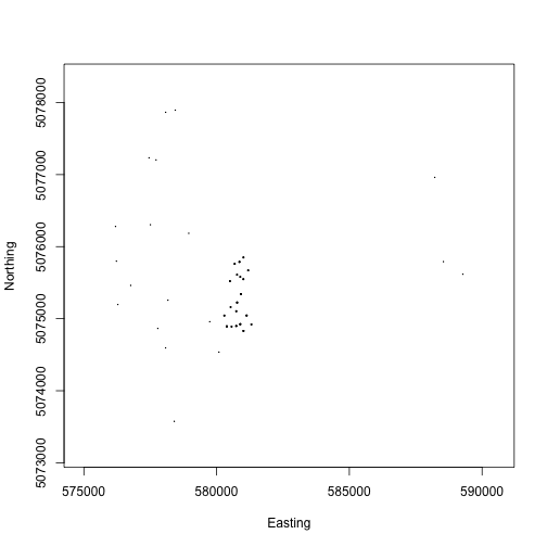
We can see where the plots are located across the landscape, and we can see the denser cluster of plots in the area near the micrometeorology tower.
For many analyses, this level of spatial data may be sufficient. Calculating the precise location of each tree is only required for certain hypotheses; consider whether you need these data when working with a data product with plot-level spatial data.
Looking back at the variables_10098 table, notice that there is
a table in this data product called vst_mappingandtagging,
suggesting we can find mapping data there. Let's take a look.
View(vst$vst_mappingandtagging)
Here we see data fields for stemDistance and stemAzimuth. Looking
back at the variables_10098 file, we see these fields contain the
distance and azimuth from a pointID to a specific stem. To calculate
the precise coordinates of each tree, we would need to get the locations
of the pointIDs, and then adjust the coordinates based on distance and
azimuth. The Data Product User Guide describes how to carry out these
steps, and can be downloaded from the
Data Product Details page.
However, carrying out these calculations yourself is not the only option!
The geoNEON package contains a function that can do this for you, for
the TOS data products with location data more precise than the plot level.
Sampling locations
The getLocTOS() function in the geoNEON package uses the NEON API to
access NEON location data and then makes protocol-specific calculations
to return precise locations for each sampling effort. This function works for a
subset of NEON TOS data products. The list of tables and data products that can
be entered is in the
package documentation on GitHub.
For more information about the NEON API, see the API tutorial and the API web page. For more information about the location calculations used in each data product, see the Data Product User Guide for each product.
The getLocTOS() function requires two inputs:
- A data table that contains spatial data from a NEON TOS data product
- The NEON table name of that data table
For vegetation structure locations, the function call looks like this. This function may take a while to download all the location data. For faster downloads, use an API token.
# calculate individual tree locations
vst.loc <- getLocTOS(data=vst$vst_mappingandtagging,
dataProd="vst_mappingandtagging")
What additional data are now available in the data obtained by getLocTOS()?
# print variable names that are new
names(vst.loc)[which(!names(vst.loc) %in%
names(vst$vst_mappingandtagging))]
## [1] "utmZone" "adjNorthing" "adjEasting"
## [4] "adjCoordinateUncertainty" "adjDecimalLatitude" "adjDecimalLongitude"
## [7] "adjElevation" "adjElevationUncertainty"
Now we have adjusted latitude, longitude, and elevation, and the corresponding easting and northing UTM data. We also have coordinate uncertainty data for these coordinates.
As we did with the plots above, we can use the easting and northing data to plot the locations of the individual trees.
plot(vst.loc$adjEasting, vst.loc$adjNorthing,
pch=".", xlab="Easting", ylab="Northing")
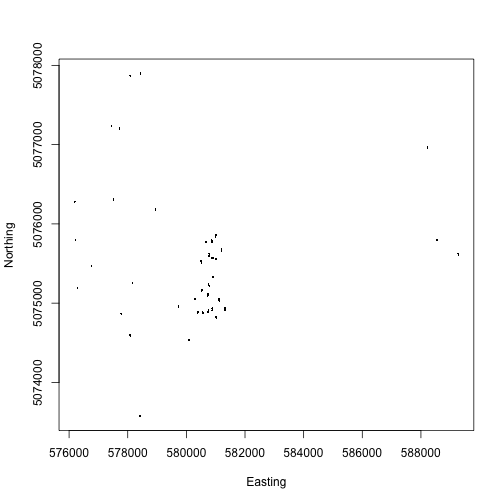
We can see the mapped trees in the same plots we mapped above.
We've plotted each individual tree as a ., so all we can see at
this scale is the cluster of dots that make up each plot.
Let's zoom in on a single plot:
plot(vst.loc$adjEasting[which(vst.loc$plotID=="WREF_085")],
vst.loc$adjNorthing[which(vst.loc$plotID=="WREF_085")],
pch=20, xlab="Easting", ylab="Northing")
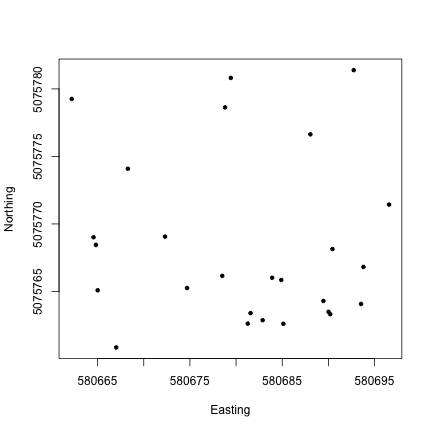
Now we can see the location of each tree within the sampling plot WREF_085. This is interesting, but it would be more interesting if we could see more information about each tree. How are species distributed across the plot, for instance?
We can plot the tree species at each location using the text() function
and the vst.loc$taxonID field.
plot(vst.loc$adjEasting[which(vst.loc$plotID=="WREF_085")],
vst.loc$adjNorthing[which(vst.loc$plotID=="WREF_085")],
type="n", xlab="Easting", ylab="Northing")
text(vst.loc$adjEasting[which(vst.loc$plotID=="WREF_085")],
vst.loc$adjNorthing[which(vst.loc$plotID=="WREF_085")],
labels=vst.loc$taxonID[which(vst.loc$plotID=="WREF_085")],
cex=0.5)
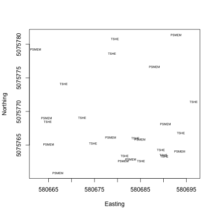
Almost all of the mapped trees in this plot are either Pseudotsuga menziesii or Tsuga heterophylla (Douglas fir and Western hemlock), not too surprising at Wind River.
But suppose we want to map the diameter of each tree? This is a very common way to present a stem map, it gives a visual as if we were looking down on the plot from overhead and had cut off each tree at its measurement height.
Other than taxon, the attributes of the trees, such as diameter, height,
growth form, and canopy position, are found in the vst_apparentindividual
table, not in the vst_mappingandtagging table. We'll need to join the
two tables to get the tree attributes together with their mapped locations.
The neonOS package contains the function joinTableNEON(), which can be
used to do this. See the tutorial for the neonOS package for more details
about this function.
veg <- joinTableNEON(vst.loc,
vst$vst_apparentindividual,
name1="vst_mappingandtagging",
name2="vst_apparentindividual")
Now we can use the symbols() function to plot the diameter of each tree,
at its spatial coordinates, to create a correctly scaled map of boles in
the plot. Note that stemDiameter is in centimeters, while easting and
northing UTMs are in meters, so we divide by 100 to scale correctly.
symbols(veg$adjEasting[which(veg$plotID=="WREF_085")],
veg$adjNorthing[which(veg$plotID=="WREF_085")],
circles=veg$stemDiameter[which(veg$plotID=="WREF_085")]/100/2,
inches=F, xlab="Easting", ylab="Northing")
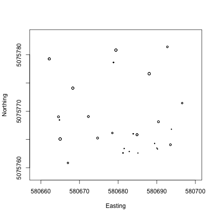
If you are interested in taking the vegetation structure data a step further, and connecting measurements of trees on the ground to remotely sensed Lidar data, check out the Vegetation Structure and Canopy Height Model tutorial.
If you are interested in working with other terrestrial observational (TOS) data products, the basic techniques used here to find precise sampling locations and join data tables can be adapted to other TOS data products. Consult the Data Product User Guide for each data product to find details specific to that data product.
Locations for sensor data
Downloads of instrument system (IS) data include a file called sensor_positions.csv. The sensor positions file contains information about the coordinates of each sensor, relative to a reference location.
While the specifics vary, techniques are generalizable for working with sensor
data and the sensor_positions.csv file. For this tutorial, let's look at the
sensor locations for soil temperature (PAR; DP1.00041.001) at
the NEON Treehaven site (TREE) in July 2018. To reduce our file size, we'll use
the 30 minute averaging interval. Our final product from this section is to
create a depth profile of soil temperature in one soil plot.
If downloading data using the neonUtilties package is new to you, check out the
neonUtilities tutorial.
This function will download about 7 MB of data as written so we have check.size =F
for ease of running the code.
# load soil temperature data of interest
soilT <- loadByProduct(dpID="DP1.00041.001", site="TREE",
startdate="2018-07", enddate="2018-07",
timeIndex=30, check.size=F)
## Attempting to stack soil sensor data. Note that due to the number of soil sensors at each site, data volume is very high for these data. Consider dividing data processing into chunks, using the nCores= parameter to parallelize stacking, and/or using a high-performance system.
Sensor positions file
Now we can specifically look at the sensor positions file.
# create object for sensor positions file
pos <- soilT$sensor_positions_00041
# view column names
names(pos)
## [1] "siteID" "HOR.VER"
## [3] "sensorLocationID" "sensorLocationDescription"
## [5] "positionStartDateTime" "positionEndDateTime"
## [7] "referenceLocationID" "referenceLocationIDDescription"
## [9] "referenceLocationIDStartDateTime" "referenceLocationIDEndDateTime"
## [11] "xOffset" "yOffset"
## [13] "zOffset" "pitch"
## [15] "roll" "azimuth"
## [17] "locationReferenceLatitude" "locationReferenceLongitude"
## [19] "locationReferenceElevation" "eastOffset"
## [21] "northOffset" "xAzimuth"
## [23] "yAzimuth" "publicationDate"
# view table
View(pos)
The sensor locations are indexed by the HOR.VER variable - see the
file naming conventions
page for more details.
Using unique() we can view all the location indices in this file.
unique(pos$HOR.VER)
## [1] "001.501" "001.502" "001.503" "001.504" "001.505" "001.506" "001.507" "001.508" "001.509" "002.501"
## [11] "002.502" "002.503" "002.504" "002.505" "002.506" "002.507" "002.508" "002.509" "003.501" "003.502"
## [21] "003.503" "003.504" "003.505" "003.506" "003.507" "003.508" "003.509" "004.501" "004.502" "004.503"
## [31] "004.504" "004.505" "004.506" "004.507" "004.508" "004.509" "005.501" "005.502" "005.503" "005.504"
## [41] "005.505" "005.506" "005.507" "005.508" "005.509"
Soil temperature data are collected in 5 instrumented soil plots inside the tower footprint. We see this reflected in the data where HOR = 001 to 005. Within each plot, temperature is measured at 9 depths, seen in VER = 501 to 509. At some sites, the number of depths may differ slightly.
The x, y, and z offsets in the sensor positions file are the relative distance, in meters, to the reference latitude, longitude, and elevation in the file.
The HOR and VER indices in the sensor positions file correspond to the
verticalPosition and horizontalPosition fields in soilT$ST_30_minute.
Note that there are two sets of position data for soil plot 001, and that
one set has a positionEndDateTime date in the file. This indicates sensors either
moved or were relocated; in this case there was a frost heave incident.
You can read about it in the issue log, which is displayed on the
Data Product Details page,
and also included as a table in the data download:
soilT$issueLog_00041[grep("TREE soil plot 1",
soilT$issueLog_00041$locationAffected),]
## id parentIssueID issueDate resolvedDate dateRangeStart dateRangeEnd
## 1: 9328 NA 2019-05-23T00:00:00Z 2019-05-23T00:00:00Z 2018-11-07T00:00:00Z 2019-04-19T00:00:00Z
## locationAffected
## 1: D05 TREE soil plot 1 measurement levels 1-9 (HOR.VER: 001.501, 001.502, 001.503, 001.504, 001.505, 001.506, 001.507, 001.508, 001.509)
## issue
## 1: Soil temperature sensors were pushed or pulled out of the ground by 3 cm over winter, presumably due to freeze-thaw action. The exact timing of this is unknown, but it occurred sometime between 2018-11-07 and 2019-04-19.
## resolution
## 1: Sensor depths were updated in the database with a start date of 2018-11-07 for the new depths.
Since we're working with data from July 2018, and the change in
sensor locations is dated Nov 2018, we'll use the original locations.
There are a number of ways to drop the later locations from the
table; here, we find the rows in which the positionEndDateTime field is empty,
indicating no end date, and the rows corresponding to soil plot 001,
and drop all the rows that meet both criteria.
pos <- pos[-intersect(grep("001.", pos$HOR.VER),
which(pos$positionEndDateTime=="")),]
Our goal is to plot a time series of temperature, stratified by depth, so let's start by joining the data file and sensor positions file, to bring the depth measurements into the same data frame with the data.
# paste horizontalPosition and verticalPosition together
# to match HOR.VER in the sensor positions file
soilT$ST_30_minute$HOR.VER <- paste(soilT$ST_30_minute$horizontalPosition,
soilT$ST_30_minute$verticalPosition,
sep=".")
# left join to keep all temperature records
soilTHV <- merge(soilT$ST_30_minute, pos,
by="HOR.VER", all.x=T)
And now we can plot soil temperature over time for each depth.
We'll use ggplot since it's well suited to this kind of
stratification. Each soil plot is its own panel, and each depth
is its own line:
gg <- ggplot(soilTHV,
aes(endDateTime, soilTempMean,
group=zOffset, color=zOffset)) +
geom_line() +
facet_wrap(~horizontalPosition)
gg
## Warning: Removed 1488 rows containing missing values (`geom_line()`).
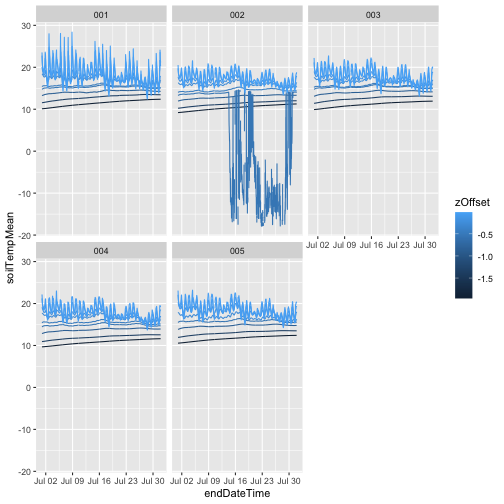
We can see that as soil depth increases, temperatures
become much more stable, while the shallowest measurement
has a clear diurnal cycle. We can also see that
something has gone wrong with one of the sensors in plot
002. To remove those data, use only values where the final
quality flag passed, i.e. finalQF = 0
gg <- ggplot(subset(soilTHV, finalQF==0),
aes(endDateTime, soilTempMean,
group=zOffset, color=zOffset)) +
geom_line() +
facet_wrap(~horizontalPosition)
gg
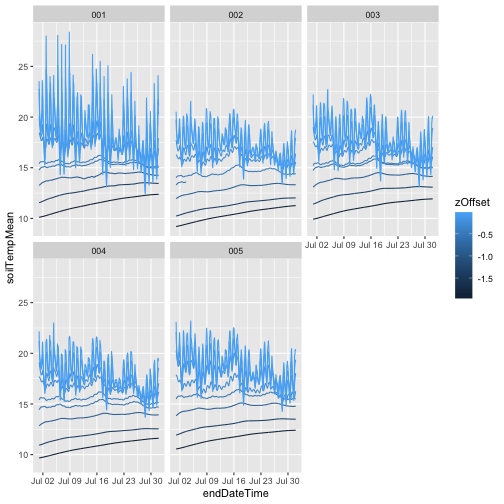
Get Lesson Code
Work With NEON's Plant Phenology Data
Last Updated: Apr 2, 2026
Many organisms, including plants, show patterns of change across seasons - the different stages of this observable change are called phenophases. In this tutorial we explore how to work with NEON plant phenophase data.
Objectives
After completing this activity, you will be able to:
- work with NEON Plant Phenology Observation data.
- use dplyr functions to filter data.
- plot time series data in a bar plot using ggplot the function.
Things You’ll Need To Complete This Tutorial
You will need the most current version of R and, preferably, RStudio loaded
on your computer to complete this tutorial.
Install R Packages
-
neonUtilities:
install.packages("neonUtilities") -
ggplot2:
install.packages("ggplot2") -
dplyr:
install.packages("dplyr")
More on Packages in R – Adapted from Software Carpentry.
Download Data
This tutorial is designed to have you download data directly from the NEON
portal API using the neonUtilities package. However, you can also directly
download this data, prepackaged, from FigShare. This data set includes all the
files needed for the Work with NEON OS & IS Data - Plant Phenology & Temperature
tutorial series. The data are in the format you would receive if downloading them
using the zipsByProduct() function in the neonUtilities package.
Additional Resources
- NEON data portal
- NEON Plant Phenology Observations data product user guide
- RStudio's data wrangling (dplyr/tidyr) cheatsheet
- NEONScience GitHub Organization
- nneo API wrapper on CRAN
Plants change throughout the year - these are phenophases. Why do they change?
Explore Phenology Data
The following sections provide a brief overview of the NEON plant phenology observation data. When designing a research project using this data, you need to consult the documents associated with this data product and not rely solely on this summary.
The following description of the NEON Plant Phenology Observation data is modified from the data product user guide.
NEON Plant Phenology Observation Data
NEON collects plant phenology data and provides it as NEON data product DP1.10055.001.
The plant phenology observations data product provides in-situ observations of the phenological status and intensity of tagged plants (or patches) during discrete observations events.
Sampling occurs at all terrestrial field sites at site and season specific intervals. During Phase I (dominant species) sampling (pre-2021), three species with 30 individuals each are sampled. In 2021, Phase II (community) sampling will begin, with <=20 species with 5 or more individuals sampled will occur.
Status-based Monitoring
NEON employs status-based monitoring, in which the phenological condition of an individual is reported any time that individual is observed. At every observations bout, records are generated for every phenophase that is occurring and for every phenophase not occurring. With this approach, events (such as leaf emergence in Mediterranean zones, or flowering in many desert species) that may occur multiple times during a single year, can be captured. Continuous reporting of phenophase status enables quantification of the duration of phenophases rather than just their date of onset while allows enabling the explicit quantification of uncertainty in phenophase transition dates that are introduced by monitoring in discrete temporal bouts.
Specific products derived from this sampling include the observed phenophase status (whether or not a phenophase is occurring) and the intensity of phenophases for individuals in which phenophase status = ‘yes’. Phenophases reported are derived from the USA National Phenology Network (USA-NPN) categories. The number of phenophases observed varies by growth form and ranges from 1 phenophase (cactus) to 7 phenophases (semi-evergreen broadleaf). In this tutorial we will focus only on the state of the phenophase, not the phenophase intensity data.
Phenology Transects
Plant phenology observations occurs at all terrestrial NEON sites along an 800 meter square loop transect (primary) and within a 200 m x 200 m plot located within view of a canopy level, tower-mounted, phenology camera.
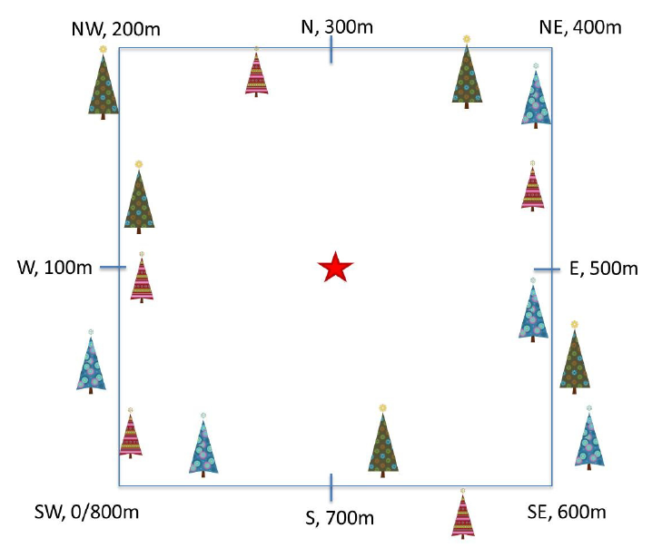
Timing of Observations
At each site, there are:
- ~50 observation bouts per year.
- no more that 100 sampling points per phenology transect.
- no more than 9 sampling points per phenocam plot.
- 1 annual measurement per year to collect annual size and disease status measurements from each sampling point.
Available Data Tables
In the downloaded data packet, data are available in two main files
- phe_statusintensity: Plant phenophase status and intensity data
- phe_perindividual: Geolocation and taxonomic identification for phenology plants
- phe_perindividualperyear: recorded once a year, essentially the "metadata" about the plant: DBH, height, etc.
There are other files in each download including a readme with information on the data product and the download; a variables file that defines the term descriptions, data types, and units; a validation file with data entry validation and parsing rules; and an XML with machine readable metadata.
Stack NEON Data
NEON data are delivered in a site and year-month format. When you download data, you will get a single zipped file containing a directory for each month and site that you've requested data for. Dealing with these separate tables from even one or two sites over a 12 month period can be a bit overwhelming. Luckily NEON provides an R package neonUtilities that takes the unzipped downloaded file and joining the data files. The teaching data downloaded with this tutorial is already stacked. If you are working with other NEON data, please go through the tutorial to stack the data in R or in Python and then return to this tutorial.
Work with NEON Data
When we do this for phenology data we get three files, one for each data table, with all the data from your site and date range of interest.
First, we need to set up our R environment.
# install needed package (only uncomment & run if not already installed)
#install.packages("neonUtilities")
#install.packages("dplyr")
#install.packages("ggplot2")
# load needed packages
library(neonUtilities)
library(dplyr)
library(ggplot2)
options(stringsAsFactors=F) #keep strings as character type not factors
# set working directory to ensure R can find the file we wish to import and where
# we want to save our files. Be sure to move the download into your working directory!
wd <- "~/Git/data/" # Change this to match your local environment
setwd(wd)
Let's start by loading our data of interest. For this series, we'll work with date from the NEON Domain 02 sites:
- Blandy Farm (BLAN)
- Smithsonian Conservation Biology Institute (SCBI)
- Smithsonian Environmental Research Center (SERC)
And we'll use data from January 2017 to December 2019. This downloads over 9MB of data. If this is too large, use a smaller date range. If you opt to do this, your figures and some output may look different later in the tutorial.
With this information, we can download our data using the neonUtilities package.
If you are not using a NEON token to download your data, remove the
token = Sys.getenv(NEON_TOKEN) line of code (learn more about NEON API tokens
in the
Using an API Token when Accessing NEON Data with neonUtilities tutorial).
If you are using the data downloaded at the start of the tutorial, use the commented out code in the second half of this code chunk.
## Two options for accessing data - programmatic or from the example dataset
# Read data from data portal
phe <- loadByProduct(dpID = "DP1.10055.001", site=c("BLAN","SCBI","SERC"),
startdate = "2017-01", enddate="2019-12",
token = Sys.getenv("NEON_TOKEN"),
check.size = F)
## API token was not recognized. Public rate limit applied.
## Finding available files
##
|
| | 0%
|
|= | 1%
|
|= | 2%
|
|== | 3%
|
|=== | 4%
|
|=== | 5%
|
|==== | 6%
|
|==== | 7%
|
|===== | 8%
|
|====== | 9%
|
|====== | 11%
|
|======= | 12%
|
|======== | 13%
|
|======== | 14%
|
|========= | 15%
|
|========== | 16%
|
|========== | 17%
|
|=========== | 18%
|
|============ | 19%
|
|============ | 20%
|
|============= | 21%
|
|============= | 22%
|
|============== | 23%
|
|=============== | 24%
|
|=============== | 25%
|
|================ | 26%
|
|================= | 27%
|
|================= | 28%
|
|================== | 29%
|
|=================== | 31%
|
|=================== | 32%
|
|==================== | 33%
|
|===================== | 34%
|
|===================== | 35%
|
|====================== | 36%
|
|====================== | 37%
|
|======================= | 38%
|
|======================== | 39%
|
|======================== | 40%
|
|========================= | 41%
|
|========================== | 42%
|
|========================== | 43%
|
|=========================== | 44%
|
|============================ | 45%
|
|============================ | 46%
|
|============================= | 47%
|
|============================== | 48%
|
|============================== | 49%
|
|=============================== | 51%
|
|=============================== | 52%
|
|================================ | 53%
|
|================================= | 54%
|
|================================= | 55%
|
|================================== | 56%
|
|=================================== | 57%
|
|=================================== | 58%
|
|==================================== | 59%
|
|===================================== | 60%
|
|===================================== | 61%
|
|====================================== | 62%
|
|======================================= | 63%
|
|======================================= | 64%
|
|======================================== | 65%
|
|======================================== | 66%
|
|========================================= | 67%
|
|========================================== | 68%
|
|========================================== | 69%
|
|=========================================== | 71%
|
|============================================ | 72%
|
|============================================ | 73%
|
|============================================= | 74%
|
|============================================== | 75%
|
|============================================== | 76%
|
|=============================================== | 77%
|
|================================================ | 78%
|
|================================================ | 79%
|
|================================================= | 80%
|
|================================================= | 81%
|
|================================================== | 82%
|
|=================================================== | 83%
|
|=================================================== | 84%
|
|==================================================== | 85%
|
|===================================================== | 86%
|
|===================================================== | 87%
|
|====================================================== | 88%
|
|======================================================= | 89%
|
|======================================================= | 91%
|
|======================================================== | 92%
|
|========================================================= | 93%
|
|========================================================= | 94%
|
|========================================================== | 95%
|
|========================================================== | 96%
|
|=========================================================== | 97%
|
|============================================================ | 98%
|
|============================================================ | 99%
|
|=============================================================| 100%
##
## Downloading files totaling approximately 7.985319 MB
## Downloading 95 files
##
|
| | 0%
|
|= | 1%
|
|= | 2%
|
|== | 3%
|
|=== | 4%
|
|=== | 5%
|
|==== | 6%
|
|===== | 7%
|
|===== | 9%
|
|====== | 10%
|
|====== | 11%
|
|======= | 12%
|
|======== | 13%
|
|======== | 14%
|
|========= | 15%
|
|========== | 16%
|
|========== | 17%
|
|=========== | 18%
|
|============ | 19%
|
|============ | 20%
|
|============= | 21%
|
|============== | 22%
|
|============== | 23%
|
|=============== | 24%
|
|================ | 26%
|
|================ | 27%
|
|================= | 28%
|
|================== | 29%
|
|================== | 30%
|
|=================== | 31%
|
|=================== | 32%
|
|==================== | 33%
|
|===================== | 34%
|
|===================== | 35%
|
|====================== | 36%
|
|======================= | 37%
|
|======================= | 38%
|
|======================== | 39%
|
|========================= | 40%
|
|========================= | 41%
|
|========================== | 43%
|
|=========================== | 44%
|
|=========================== | 45%
|
|============================ | 46%
|
|============================= | 47%
|
|============================= | 48%
|
|============================== | 49%
|
|============================== | 50%
|
|=============================== | 51%
|
|================================ | 52%
|
|================================ | 53%
|
|================================= | 54%
|
|================================== | 55%
|
|================================== | 56%
|
|=================================== | 57%
|
|==================================== | 59%
|
|==================================== | 60%
|
|===================================== | 61%
|
|====================================== | 62%
|
|====================================== | 63%
|
|======================================= | 64%
|
|======================================== | 65%
|
|======================================== | 66%
|
|========================================= | 67%
|
|========================================== | 68%
|
|========================================== | 69%
|
|=========================================== | 70%
|
|=========================================== | 71%
|
|============================================ | 72%
|
|============================================= | 73%
|
|============================================= | 74%
|
|============================================== | 76%
|
|=============================================== | 77%
|
|=============================================== | 78%
|
|================================================ | 79%
|
|================================================= | 80%
|
|================================================= | 81%
|
|================================================== | 82%
|
|=================================================== | 83%
|
|=================================================== | 84%
|
|==================================================== | 85%
|
|===================================================== | 86%
|
|===================================================== | 87%
|
|====================================================== | 88%
|
|======================================================= | 89%
|
|======================================================= | 90%
|
|======================================================== | 91%
|
|======================================================== | 93%
|
|========================================================= | 94%
|
|========================================================== | 95%
|
|========================================================== | 96%
|
|=========================================================== | 97%
|
|============================================================ | 98%
|
|============================================================ | 99%
|
|=============================================================| 100%
##
## Unpacking zip files using 1 cores.
## Stacking operation across a single core.
## Stacking table phe_perindividual
## Stacking table phe_statusintensity
## Stacking table phe_perindividualperyear
## Copied the most recent publication of validation file to /stackedFiles
## Copied the most recent publication of categoricalCodes file to /stackedFiles
## Copied the most recent publication of variable definition file to /stackedFiles
## Finished: Stacked 3 data tables and 3 metadata tables!
## Stacking took 1.46806 secs
# if you aren't sure you can handle the data file size use check.size = T.
# save dataframes from the downloaded list
ind <- phe$phe_perindividual #individual information
status <- phe$phe_statusintensity #status & intensity info
##If choosing to use example dataset downloaded from this tutorial:
# Stack multiple files within the downloaded phenology data
#stackByTable("NEON-pheno-temp-timeseries_v2/filesToStack10055", folder = T)
# read in data - readTableNEON uses the variables file to assign the correct
# data type for each variable
#ind <- readTableNEON('NEON-pheno-temp-timeseries_v2/filesToStack10055/stackedFiles/phe_perindividual.csv', 'NEON-pheno-temp-timeseries_v2/filesToStack10055/stackedFiles/variables_10055.csv')
#status <- readTableNEON('NEON-pheno-temp-timeseries_v2/filesToStack10055/stackedFiles/phe_statusintensity.csv', 'NEON-pheno-temp-timeseries_v2/filesToStack10055/stackedFiles/variables_10055.csv')
Let's explore the data. Let's get to know what the ind dataframe looks like.
# What are the fieldnames in this dataset?
names(ind)
## [1] "uid" "namedLocation"
## [3] "domainID" "siteID"
## [5] "plotID" "decimalLatitude"
## [7] "decimalLongitude" "geodeticDatum"
## [9] "coordinateUncertainty" "elevation"
## [11] "elevationUncertainty" "subtypeSpecification"
## [13] "transectMeter" "directionFromTransect"
## [15] "ninetyDegreeDistance" "sampleLatitude"
## [17] "sampleLongitude" "sampleGeodeticDatum"
## [19] "sampleCoordinateUncertainty" "sampleElevation"
## [21] "sampleElevationUncertainty" "date"
## [23] "editedDate" "individualID"
## [25] "taxonID" "scientificName"
## [27] "identificationQualifier" "taxonRank"
## [29] "nativeStatusCode" "growthForm"
## [31] "vstTag" "samplingProtocolVersion"
## [33] "measuredBy" "identifiedBy"
## [35] "recordedBy" "remarks"
## [37] "dataQF" "publicationDate"
## [39] "release"
# Unsure of what some of the variables are you? Look at the variables table!
View(phe$variables_10055)
# if using the pre-downloaded data, you need to read in the variables file
# or open and look at it on your desktop
#var <- read.csv('NEON-pheno-temp-timeseries_v2/filesToStack10055/stackedFiles/variables_10055.csv')
#View(var)
# how many rows are in the data?
nrow(ind)
## [1] 433
# look at the first six rows of data.
#head(ind) #this is a good function to use but looks messy so not rendering it
# look at the structure of the dataframe.
str(ind)
## 'data.frame': 433 obs. of 39 variables:
## $ uid : chr "76bf37d9-c834-43fc-a430-83d87e4b9289" "cf0239bb-2953-44a8-8fd2-051539be5727" "833e5f41-d5cb-4550-ba60-e6f000a2b1b6" "6c2e348d-d19e-4543-9d22-0527819ee964" ...
## $ namedLocation : chr "BLAN_061.phenology.phe" "BLAN_061.phenology.phe" "BLAN_061.phenology.phe" "BLAN_061.phenology.phe" ...
## $ domainID : chr "D02" "D02" "D02" "D02" ...
## $ siteID : chr "BLAN" "BLAN" "BLAN" "BLAN" ...
## $ plotID : chr "BLAN_061" "BLAN_061" "BLAN_061" "BLAN_061" ...
## $ decimalLatitude : num 39.1 39.1 39.1 39.1 39.1 ...
## $ decimalLongitude : num -78.1 -78.1 -78.1 -78.1 -78.1 ...
## $ geodeticDatum : chr NA NA NA NA ...
## $ coordinateUncertainty : num NA NA NA NA NA NA NA NA NA NA ...
## $ elevation : num 183 183 183 183 183 183 183 183 183 183 ...
## $ elevationUncertainty : num NA NA NA NA NA NA NA NA NA NA ...
## $ subtypeSpecification : chr "primary" "primary" "primary" "primary" ...
## $ transectMeter : num 491 464 537 15 753 506 527 305 627 501 ...
## $ directionFromTransect : chr "Left" "Right" "Left" "Left" ...
## $ ninetyDegreeDistance : num 0.5 4 2 3 2 1 2 3 2 3 ...
## $ sampleLatitude : num NA NA NA NA NA NA NA NA NA NA ...
## $ sampleLongitude : num NA NA NA NA NA NA NA NA NA NA ...
## $ sampleGeodeticDatum : chr "WGS84" "WGS84" "WGS84" "WGS84" ...
## $ sampleCoordinateUncertainty: num NA NA NA NA NA NA NA NA NA NA ...
## $ sampleElevation : num NA NA NA NA NA NA NA NA NA NA ...
## $ sampleElevationUncertainty : num NA NA NA NA NA NA NA NA NA NA ...
## $ date : POSIXct, format: "2016-04-20" ...
## $ editedDate : POSIXct, format: "2016-05-09" ...
## $ individualID : chr "NEON.PLA.D02.BLAN.06290" "NEON.PLA.D02.BLAN.06501" "NEON.PLA.D02.BLAN.06204" "NEON.PLA.D02.BLAN.06223" ...
## $ taxonID : chr "RHDA" "SOAL6" "RHDA" "LOMA6" ...
## $ scientificName : chr "Rhamnus davurica Pall." "Solidago altissima L." "Rhamnus davurica Pall." "Lonicera maackii (Rupr.) Herder" ...
## $ identificationQualifier : chr NA NA NA NA ...
## $ taxonRank : chr "species" "species" "species" "species" ...
## $ nativeStatusCode : chr "I" "N" "I" "I" ...
## $ growthForm : chr "Deciduous broadleaf" "Forb" "Deciduous broadleaf" "Deciduous broadleaf" ...
## $ vstTag : chr NA NA NA NA ...
## $ samplingProtocolVersion : chr NA "NEON.DOC.014040vJ" "NEON.DOC.014040vJ" "NEON.DOC.014040vJ" ...
## $ measuredBy : chr "jcoloso@neoninc.org" "jward@battelleecology.org" "alandes@field-ops.org" "alandes@field-ops.org" ...
## $ identifiedBy : chr "shackley@neoninc.org" "llemmon@field-ops.org" "llemmon@field-ops.org" "llemmon@field-ops.org" ...
## $ recordedBy : chr "shackley@neoninc.org" NA NA NA ...
## $ remarks : chr "Nearly dead shaded out" "no entry" "no entry" "no entry" ...
## $ dataQF : chr NA NA NA NA ...
## $ publicationDate : chr "20201218T103411Z" "20201218T103411Z" "20201218T103411Z" "20201218T103411Z" ...
## $ release : chr "RELEASE-2021" "RELEASE-2021" "RELEASE-2021" "RELEASE-2021" ...
Notice that the neonUtilities package read the data type from the variables file and then automatically converts the data to the correct date type in R.
(Note that if you first opened your data file in Excel, you might see 06/14/2014 as the format instead of 2014-06-14. Excel can do some ~~weird~~ interesting things to dates.)
Phenology status
Now let's look at the status data.
# What variables are included in this dataset?
names(status)
## [1] "uid" "namedLocation"
## [3] "domainID" "siteID"
## [5] "plotID" "date"
## [7] "editedDate" "dayOfYear"
## [9] "individualID" "phenophaseName"
## [11] "phenophaseStatus" "phenophaseIntensityDefinition"
## [13] "phenophaseIntensity" "samplingProtocolVersion"
## [15] "measuredBy" "recordedBy"
## [17] "remarks" "dataQF"
## [19] "publicationDate" "release"
nrow(status)
## [1] 219357
#head(status) #this is a good function to use but looks messy so not rendering it
str(status)
## 'data.frame': 219357 obs. of 20 variables:
## $ uid : chr "b69ada55-41d1-41c7-9031-149c54de51f9" "9be6f7ad-4422-40ac-ba7f-e32e0184782d" "58e7aeaf-163c-4ea2-ad75-db79a580f2f8" "efe7ca02-d09e-4964-b35d-aebdac8f3efb" ...
## $ namedLocation : chr "BLAN_061.phenology.phe" "BLAN_061.phenology.phe" "BLAN_061.phenology.phe" "BLAN_061.phenology.phe" ...
## $ domainID : chr "D02" "D02" "D02" "D02" ...
## $ siteID : chr "BLAN" "BLAN" "BLAN" "BLAN" ...
## $ plotID : chr "BLAN_061" "BLAN_061" "BLAN_061" "BLAN_061" ...
## $ date : POSIXct, format: "2017-02-24" ...
## $ editedDate : POSIXct, format: "2017-03-31" ...
## $ dayOfYear : num 55 55 55 55 55 55 55 55 55 55 ...
## $ individualID : chr "NEON.PLA.D02.BLAN.06229" "NEON.PLA.D02.BLAN.06226" "NEON.PLA.D02.BLAN.06222" "NEON.PLA.D02.BLAN.06223" ...
## $ phenophaseName : chr "Leaves" "Leaves" "Leaves" "Leaves" ...
## $ phenophaseStatus : chr "no" "no" "no" "no" ...
## $ phenophaseIntensityDefinition: chr NA NA NA NA ...
## $ phenophaseIntensity : chr NA NA NA NA ...
## $ samplingProtocolVersion : chr NA NA NA NA ...
## $ measuredBy : chr "llemmon@neoninc.org" "llemmon@neoninc.org" "llemmon@neoninc.org" "llemmon@neoninc.org" ...
## $ recordedBy : chr "llemmon@neoninc.org" "llemmon@neoninc.org" "llemmon@neoninc.org" "llemmon@neoninc.org" ...
## $ remarks : chr NA NA NA NA ...
## $ dataQF : chr "legacyData" "legacyData" "legacyData" "legacyData" ...
## $ publicationDate : chr "20201217T203824Z" "20201217T203824Z" "20201217T203824Z" "20201217T203824Z" ...
## $ release : chr "RELEASE-2021" "RELEASE-2021" "RELEASE-2021" "RELEASE-2021" ...
# date range
min(status$date)
## [1] "2017-02-24 GMT"
max(status$date)
## [1] "2019-12-12 GMT"
Clean up the Data
- remove duplicates (full rows)
- convert to date format
- retain only the most recent
editedDatein the perIndividual and status table.
Remove Duplicates
The individual table (ind) file is included in each site by month-year file. As a result when all the tables are stacked there are many duplicates.
Let's remove any duplicates that exist.
# drop UID as that will be unique for duplicate records
ind_noUID <- select(ind, -(uid))
status_noUID <- select(status, -(uid))
# remove duplicates
## expect many
ind_noD <- distinct(ind_noUID)
nrow(ind_noD)
## [1] 433
status_noD<-distinct(status_noUID)
nrow(status_noD)
## [1] 216837
Variable Overlap between Tables
From the initial inspection of the data we can see there is overlap in variable names between the fields.
Let's see what they are.
# where is there an intersection of names
intersect(names(status_noD), names(ind_noD))
## [1] "namedLocation" "domainID"
## [3] "siteID" "plotID"
## [5] "date" "editedDate"
## [7] "individualID" "samplingProtocolVersion"
## [9] "measuredBy" "recordedBy"
## [11] "remarks" "dataQF"
## [13] "publicationDate" "release"
There are several fields that overlap between the datasets. Some of these are expected to be the same and will be what we join on.
However, some of these will have different values in each table. We want to keep those distinct value and not join on them. Therefore, we can rename these fields before joining:
- date
- editedDate
- measuredBy
- recordedBy
- samplingProtocolVersion
- remarks
- dataQF
- publicationDate
Now we want to rename the variables that would have duplicate names. We can rename all the variables in the status object to have "Stat" at the end of the variable name.
# in Status table rename like columns
status_noD <- rename(status_noD, dateStat=date,
editedDateStat=editedDate, measuredByStat=measuredBy,
recordedByStat=recordedBy,
samplingProtocolVersionStat=samplingProtocolVersion,
remarksStat=remarks, dataQFStat=dataQF,
publicationDateStat=publicationDate)
Filter to last editedDate
The individual (ind) table contains all instances that any of the location or
taxonomy data of an individual was updated. Therefore there are many rows for
some individuals. We only want the latest editedDate on ind.
# retain only the max of the date for each individualID
ind_last <- ind_noD %>%
group_by(individualID) %>%
filter(editedDate==max(editedDate))
# oh wait, duplicate dates, retain only the most recent editedDate
ind_lastnoD <- ind_last %>%
group_by(editedDate, individualID) %>%
filter(row_number()==1)
Join Dataframes
Now we can join the two data frames on all the variables with the same name.
We use a left_join() from the dpylr package because we want to match all the
rows from the "left" (first) dataframe to any rows that also occur in the "right"
(second) dataframe.
Check out RStudio's data wrangling (dplyr/tidyr) cheatsheet for other types of joins.
# Create a new dataframe "phe_ind" with all the data from status and some from ind_lastnoD
phe_ind <- left_join(status_noD, ind_lastnoD)
## Joining, by = c("namedLocation", "domainID", "siteID", "plotID", "individualID", "release")
Now that we have clean datasets we can begin looking into our particular data to address our research question: do plants show patterns of changes in phenophase across season?
Patterns in Phenophase
From our larger dataset (several sites, species, phenophases), let's create a
dataframe with only the data from a single site, species, and phenophase and
call it phe_1sp.
Select Site(s) of Interest
To do this, we'll first select our site of interest. Note how we set this up with an object that is our site of interest. This will allow us to more easily change which site or sites if we want to adapt our code later.
# set site of interest
siteOfInterest <- "SCBI"
# use filter to select only the site of Interest
## using %in% allows one to add a vector if you want more than one site.
## could also do it with == instead of %in% but won't work with vectors
phe_1st <- filter(phe_ind, siteID %in% siteOfInterest)
Select Species of Interest
Now we may only want to view a single species or a set of species. Let's first
look at the species that are present in our data. We could do this just by looking
at the taxonID field which give the four letter UDSA plant code for each
species. But if we don't know all the plant codes, we can get a bit fancier and
view both
# see which species are present - taxon ID only
unique(phe_1st$taxonID)
## [1] "JUNI" "MIVI" "LITU"
# or see which species are present with taxon ID + species name
unique(paste(phe_1st$taxonID, phe_1st$scientificName, sep=' - '))
## [1] "JUNI - Juglans nigra L."
## [2] "MIVI - Microstegium vimineum (Trin.) A. Camus"
## [3] "LITU - Liriodendron tulipifera L."
For now, let's choose only the flowering tree Liriodendron tulipifera (LITU).
By writing it this way, we could also add a list of species to the speciesOfInterest
object to select for multiple species.
speciesOfInterest <- "LITU"
#subset to just "LITU"
# here just use == but could also use %in%
phe_1sp <- filter(phe_1st, taxonID==speciesOfInterest)
# check that it worked
unique(phe_1sp$taxonID)
## [1] "LITU"
Select Phenophase of Interest
And, perhaps a single phenophase.
# see which phenophases are present
unique(phe_1sp$phenophaseName)
## [1] "Open flowers" "Breaking leaf buds"
## [3] "Colored leaves" "Increasing leaf size"
## [5] "Falling leaves" "Leaves"
phenophaseOfInterest <- "Leaves"
#subset to just the phenosphase of interest
phe_1sp <- filter(phe_1sp, phenophaseName %in% phenophaseOfInterest)
# check that it worked
unique(phe_1sp$phenophaseName)
## [1] "Leaves"
Select only Primary Plots
NEON plant phenology observations are collected along two types of plots.
- Primary plots: an 800 meter square phenology loop transect
- Phenocam plots: a 200 m x 200 m plot located within view of a canopy level, tower-mounted, phenology camera
In the data, these plots are differentiated by the subtypeSpecification.
Depending on your question you may want to use only one or both of these plot types.
For this activity, we're going to only look at the primary plots.
# what plots are present?
unique(phe_1sp$subtypeSpecification)
## [1] "primary" "phenocam"
# filter
phe_1spPrimary <- filter(phe_1sp, subtypeSpecification == 'primary')
# check that it worked
unique(phe_1spPrimary$subtypeSpecification)
## [1] "primary"
Total in Phenophase of Interest
The phenophaseState is recorded as "yes" or "no" that the individual is in that
phenophase. The phenophaseIntensity are categories for how much of the individual
is in that state. For now, we will stick with phenophaseState.
We can now calculate the total number of individuals with that state. We use
n_distinct(indvidualID) count the individuals (and not the records) in case
there are duplicate records for an individual.
But later on we'll also want to calculate the percent of the observed individuals in the "leaves" status, therefore, we're also adding in a step here to retain the sample size so that we can calculate % later.
Here we use pipes %>% from the dpylr package to "pass" objects onto the next
function.
# Calculate sample size for later use
sampSize <- phe_1spPrimary %>%
group_by(dateStat) %>%
summarise(numInd= n_distinct(individualID))
# Total in status by day for distinct individuals
inStat <- phe_1spPrimary%>%
group_by(dateStat, phenophaseStatus)%>%
summarise(countYes=n_distinct(individualID))
## `summarise()` has grouped output by 'dateStat'. You can override using the `.groups` argument.
inStat <- full_join(sampSize, inStat, by="dateStat")
# Retain only Yes
inStat_T <- filter(inStat, phenophaseStatus %in% "yes")
# check that it worked
unique(inStat_T$phenophaseStatus)
## [1] "yes"
Now that we have the data we can plot it.
Plot with ggplot
The ggplot() function within the ggplot2 package gives us considerable control
over plot appearance. Three basic elements are needed for ggplot() to work:
- The data_frame: containing the variables that we wish to plot,
-
aes(aesthetics): which denotes which variables will map to the x-, y- (and other) axes, -
geom_XXXX(geometry): which defines the data's graphical representation (e.g. points (geom_point), bars (geom_bar), lines (geom_line), etc).
The syntax begins with the base statement that includes the data_frame
(inStat_T) and associated x (date) and y (n) variables to be
plotted:
ggplot(inStat_T, aes(date, n))
Bar Plots with ggplot
To successfully plot, the last piece that is needed is the geometry type.
To create a bar plot, we set the geom element from to geom_bar().
The default setting for a ggplot bar plot - geom_bar() - is a histogram
designated by stat="bin". However, in this case, we want to plot count values.
We can use geom_bar(stat="identity") to force ggplot to plot actual values.
# plot number of individuals in leaf
phenoPlot <- ggplot(inStat_T, aes(dateStat, countYes)) +
geom_bar(stat="identity", na.rm = TRUE)
phenoPlot
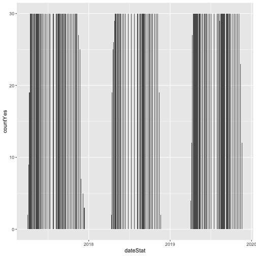
# Now let's make the plot look a bit more presentable
phenoPlot <- ggplot(inStat_T, aes(dateStat, countYes)) +
geom_bar(stat="identity", na.rm = TRUE) +
ggtitle("Total Individuals in Leaf") +
xlab("Date") + ylab("Number of Individuals") +
theme(plot.title = element_text(lineheight=.8, face="bold", size = 20)) +
theme(text = element_text(size=18))
phenoPlot
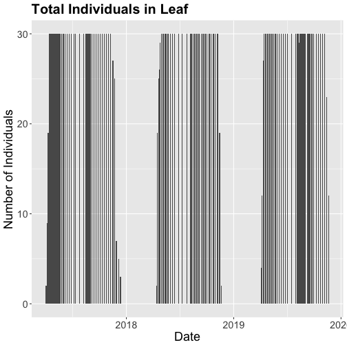
We could also covert this to percentage and plot that.
# convert to percent
inStat_T$percent<- ((inStat_T$countYes)/inStat_T$numInd)*100
# plot percent of leaves
phenoPlot_P <- ggplot(inStat_T, aes(dateStat, percent)) +
geom_bar(stat="identity", na.rm = TRUE) +
ggtitle("Proportion in Leaf") +
xlab("Date") + ylab("% of Individuals") +
theme(plot.title = element_text(lineheight=.8, face="bold", size = 20)) +
theme(text = element_text(size=18))
phenoPlot_P
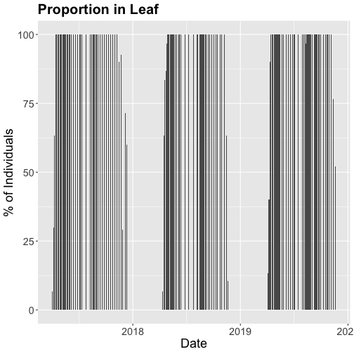
The plots demonstrate the nice expected pattern of increasing leaf-out, peak, and drop-off.
Drivers of Phenology
Now that we see that there are differences in and shifts in phenophases, what are the drivers of phenophases?
The NEON phenology measurements track sensitive and easily observed indicators of biotic responses to meteorological variability by monitoring the timing and duration of phenological stages in plant communities. Plant phenology is affected by forces such as temperature, timing and duration of pest infestations and disease outbreaks, water fluxes, nutrient budgets, carbon dynamics, and food availability and has feedbacks to trophic interactions, carbon sequestration, community composition and ecosystem function. (quoted from Plant Phenology Observations user guide.)
Filter by Date
In the next part of this series, we will be exploring temperature as a driver of phenology. Temperature date is quite large (NEON provides this in 1 minute or 30 minute intervals) so let's trim our phenology date down to only one year so that we aren't working with as large a data.
Let's filter to just 2018 data.
# use filter to select only the date of interest
phe_1sp_2018 <- filter(inStat_T, dateStat >= "2018-01-01" & dateStat <= "2018-12-31")
# did it work?
range(phe_1sp_2018$dateStat)
## [1] "2018-04-13 GMT" "2018-11-20 GMT"
How does that look?
# Now let's make the plot look a bit more presentable
phenoPlot18 <- ggplot(phe_1sp_2018, aes(dateStat, countYes)) +
geom_bar(stat="identity", na.rm = TRUE) +
ggtitle("Total Individuals in Leaf") +
xlab("Date") + ylab("Number of Individuals") +
theme(plot.title = element_text(lineheight=.8, face="bold", size = 20)) +
theme(text = element_text(size=18))
phenoPlot18
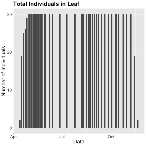
Now that we've filtered down to just the 2018 data from SCBI for LITU in leaf, we may want to save that subsetted data for another use. To do that you can write the data frame to a .csv file.
You do not need to follow this step if you are continuing on to the next tutorials in this series as you already have the data frame in your environment. Of course if you close R and then come back to it, you will need to re-load this data and instructions for that are provided in the relevant tutorials.
# Write .csv - this step is optional
# This will write to your current working directory, change as desired.
write.csv( phe_1sp_2018 , file="NEONpheno_LITU_Leaves_SCBI_2018.csv", row.names=F)
#If you are using the downloaded example date, this code will write it to the
# pheno data file. Note - this file is already a part of the download.
#write.csv( phe_1sp_2018 , file="NEON-pheno-temp-timeseries_v2/NEONpheno_LITU_Leaves_SCBI_2018.csv", row.names=F)
Get Lesson Code
Work with NEON's Single-Aspirated Air Temperature Data
Last Updated: Apr 2, 2026
In this tutorial, we explore the NEON single-aspirated air temperature data. We then discuss how to interpret the variables, how to work with date-time and date formats, and finally how to plot the data.
This tutorial is part of a series on how to work with both discrete and continuous time series data with NEON plant phenology and temperature data products.
Objectives
After completing this activity, you will be able to:
- work with "stacked" NEON Single-Aspirated Air Temperature data.
- correctly format date-time data.
- use dplyr functions to filter data.
- plot time series data in scatter plots using ggplot function.
Things You’ll Need To Complete This Tutorial
You will need the most current version of R and, preferably, RStudio loaded
on your computer to complete this tutorial.
Install R Packages
-
neonUtilities:
install.packages("neonUtilities") -
ggplot2:
install.packages("ggplot2") -
dplyr:
install.packages("dplyr") -
tidyr:
install.packages("tidyr")
More on Packages in R – Adapted from Software Carpentry.
Additional Resources
- NEON data portal
- RStudio's data wrangling (dplyr/tidyr) cheatsheet
- NEONScience GitHub Organization
- nneo API wrapper on CRAN
- RStudio's data wrangling (dplyr/tidyr) cheatsheet
- Hadley Wickham's
documentation
on the
ggplot2package. - Winston Chang's
Background Information About NEON Air Temperature Data
Air temperature is continuously monitored by NEON by two methods. At terrestrial sites temperature at the top of the tower is derived from a triple redundant aspirated air temperature sensor. This is provided as NEON data product DP1.00003.001. Single Aspirated Air Temperature sensors (SAAT) are deployed to develop temperature profiles at multiple levels on the tower at NEON terrestrial sites and on the meteorological stations at NEON aquatic sites. This is provided as NEON data product DP1.00002.001.
When designing a research project using this data, consult the Data Product Details Page for more detailed documentation.
Single-aspirated Air Temperature
Air temperature profiles are ascertained by deploying SAATs at various heights on NEON tower infrastructure. Air temperature at aquatic sites is measured using a single SAAT at a standard height of 3m above ground level. Air temperature for this data product is provided as one- and thirty-minute averages of 1 Hz observations. Temperature observations are made using platinum resistance thermometers, which are housed in a fan aspirated shield to reduce radiative heating. The temperature is measured in Ohms and subsequently converted to degrees Celsius during data processing. Details on the conversion can be found in the associated Algorithm Theoretic Basis Document (ATBD; see Product Details page linked above).
Available Data Tables
The SAAT data product contains two data tables for each site and month selected, consisting of the 1-minute and 30-minute averaging intervals. In addition, there are several metadata files that provide additional useful information.
- readme with information on the data product and the download
- variables file that defines the terms, data types, and units
- EML file with machine readable metadata in standardized Ecological Metadata Language
Access NEON Data
There are several ways to access NEON data, directly from the NEON data portal, access through a data partner (select data products only), writing code to directly pull data from the NEON API, or, as we'll do here, using the neonUtilities package which is a wrapper for the API to make working with the data easier.
Downloading from the Data Portal
If you prefer to download data from the data portal, please review the Getting started and Stack the downloaded data sections of the Download and Explore NEON Data tutorial. This will get you to the point where you can download data from sites or dates of interest and resume this tutorial.
Downloading Data Using neonUtilities
First, we need to set up our environment with the packages needed for this tutorial.
# Install needed package (only uncomment & run if not already installed)
#install.packages("neonUtilities")
#install.packages("ggplot2")
#install.packages("dplyr")
#install.packages("tidyr")
# Load required libraries
library(neonUtilities) # for accessing NEON data
library(ggplot2) # for plotting
library(dplyr) # for data munging
library(tidyr) # for data munging
# set working directory
# this step is optional, only needed if you plan to save the
# data files at the end of the tutorial
wd <- "~/data" # enter your working directory here
setwd(wd)
This tutorial is part of series working with discrete plant phenology data and (nearly) continuous temperature data. Our overall "research" question is to see if there is any correlation between plant phenology and temperature. Therefore, we will want to work with data that align with the plant phenology data that we worked with in the first tutorial. If you are only interested in working with the temperature data, you do not need to complete the previous tutorial.
Our data of interest will be the temperature data from 2018 from NEON's Smithsonian Conservation Biology Institute (SCBI) field site located in Virginia near the northern terminus of the Blue Ridge Mountains.
NEON single aspirated air temperature data is available in two averaging intervals, 1 minute and 30 minute intervals. Which data you want to work with is going to depend on your research questions. Here, we're going to only download and work with the 30 minute interval data as we're primarily interest in longer term (daily, weekly, annual) patterns.
This will download 7.7 MB of data. check.size is set to false (F) to improve flow
of the script but is always a good idea to view the size with true (T) before
downloading a new dataset.
# download data of interest - Single Aspirated Air Temperature
saat <- loadByProduct(dpID="DP1.00002.001", site="SCBI",
startdate="2018-01", enddate="2018-12",
package="basic", timeIndex="30",
check.size = F)
Explore Temperature Data
Now that you have the data, let's take a look at the structure and understand
what's in the data. The data (saat) come in as a large list of four items.
View(saat)
So what exactly are these five files and why would you want to use them?
-
data file(s): There will always be one or more dataframes that include the
primary data of the data product you downloaded. Since we downloaded only the 30
minute averaged data we only have one data table
SAAT_30min. - readme_xxxxx: The readme file, with the corresponding 5 digits from the data product number, provides you with important information relevant to the data product and the specific instance of downloading the data.
- sensor_positions_xxxxx: This table contains the spatial coordinates of each sensor, relative to a reference location.
- variables_xxxxx: This table contains all the variables found in the associated data table(s). This includes full definitions, units, and rounding.
- issueLog_xxxxx: This table contains records of any known issues with the data product, such as sensor malfunctions.
- scienceReviewFlags_xxxxx: This table may or may not be present. It contains descriptions of adverse events that led to manual flagging of the data, and is usually more detailed than the issue log. It only contains records relevant to the sites and dates of data downloaded.
Since we want to work with the individual files, let's make the elements of the list into independent objects.
list2env(saat, .GlobalEnv)
## <environment: R_GlobalEnv>
Now let's take a look at the data table.
str(SAAT_30min)
## 'data.frame': 87600 obs. of 16 variables:
## $ domainID : chr "D02" "D02" "D02" "D02" ...
## $ siteID : chr "SCBI" "SCBI" "SCBI" "SCBI" ...
## $ horizontalPosition : chr "000" "000" "000" "000" ...
## $ verticalPosition : chr "010" "010" "010" "010" ...
## $ startDateTime : POSIXct, format: "2018-01-01 00:00:00" "2018-01-01 00:30:00" "2018-01-01 01:00:00" ...
## $ endDateTime : POSIXct, format: "2018-01-01 00:30:00" "2018-01-01 01:00:00" "2018-01-01 01:30:00" ...
## $ tempSingleMean : num -11.8 -11.8 -12 -12.2 -12.4 ...
## $ tempSingleMinimum : num -12.1 -12.2 -12.3 -12.6 -12.8 ...
## $ tempSingleMaximum : num -11.4 -11.3 -11.3 -11.7 -12.1 ...
## $ tempSingleVariance : num 0.0208 0.0315 0.0412 0.0393 0.0361 0.0289 0.0126 0.0211 0.0115 0.0022 ...
## $ tempSingleNumPts : num 1800 1800 1800 1800 1800 1800 1800 1800 1800 1800 ...
## $ tempSingleExpUncert: num 0.13 0.13 0.13 0.13 0.129 ...
## $ tempSingleStdErMean: num 0.0034 0.0042 0.0048 0.0047 0.0045 0.004 0.0026 0.0034 0.0025 0.0011 ...
## $ finalQF : num 0 0 0 0 0 0 0 0 0 0 ...
## $ publicationDate : chr "20221210T185420Z" "20221210T185420Z" "20221210T185420Z" "20221210T185420Z" ...
## $ release : chr "undetermined" "undetermined" "undetermined" "undetermined" ...
Quality Flags
The sensor data undergo a variety of automated quality assurance and quality control
checks. You can read about them in detail in the Quality Flags and Quality Metrics ATBD, in the Documentation section of the product details page.
The expanded data package
includes all of these quality flags, which can allow you to decide if not passing
one of the checks will significantly hamper your research and if you should
therefore remove the data from your analysis. Here, we're using the
basic data package, which only includes the final quality flag (finalQF),
which is aggregated from the full set of quality flags.
A pass of the check is 0, while a fail is 1. Let's see what percentage of the data we downloaded passed the quality checks.
sum(SAAT_30min$finalQF==1)/nrow(SAAT_30min)
## [1] 0.2340297
What should we do with the 23% of the data that are flagged? This may depend on why it is flagged and what questions you are asking, and the expanded data package would be useful for determining this.
For now, for demonstration purposes, we'll keep the flagged data.
What about null (NA) data?
sum(is.na(SAAT_30min$tempSingleMean))/nrow(SAAT_30min)
## [1] 0.2239269
mean(SAAT_30min$tempSingleMean)
## [1] NA
22% of the mean temperature values are NA. Note that this is not
additive with the flagged data! Empty data records are flagged, so this
indicates nearly all of the flagged data in our download are empty records.
Why was there no output from the calculation of mean temperature?
The R programming language, by default, won't calculate a mean (and many other
summary statistics) in data that contain NA values. We could override this
using the input parameter na.rm=TRUE in the mean() function, or just
remove the empty values from our analysis.
# create new dataframe without NAs
SAAT_30min_noNA <- SAAT_30min %>%
drop_na(tempSingleMean) # tidyr function
# alternate base R
# SAAT_30min_noNA <- SAAT_30min[!is.na(SAAT_30min$tempSingleMean),]
# did it work?
sum(is.na(SAAT_30min_noNA$tempSingleMean))
## [1] 0
Scatterplots with ggplot
We can use ggplot to create scatter plots. Which data should we plot, as we have several options?
- tempSingleMean: the mean temperature for the interval
- tempSingleMinimum: the minimum temperature during the interval
- tempSingleMaximum: the maximum temperature for the interval
Depending on exactly what question you are asking you may prefer to use one over the other. For many applications, the mean temperature of the 1- or 30-minute interval will provide the best representation of the data.
Let's plot it. (This is a plot of a large amount of data. It can take 1-2 mins to process. It is not essential for completing the next steps if this takes too much of your computer memory.)
# plot temp data
tempPlot <- ggplot(SAAT_30min, aes(startDateTime, tempSingleMean)) +
geom_point(size=0.3) +
ggtitle("Single Aspirated Air Temperature") +
xlab("Date") + ylab("Temp (C)") +
theme(plot.title = element_text(lineheight=.8, face="bold", size = 20)) +
theme(text = element_text(size=18))
tempPlot
## Warning: Removed 19616 rows containing missing values (`geom_point()`).
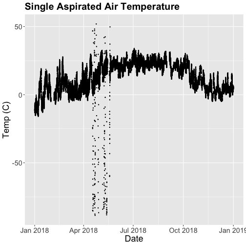
What patterns can you see in the data?
Something odd seems to have happened in late April/May 2018. Since it is unlikely Virginia experienced -50C during this time, these are probably erroneous sensor readings and why we should probably remove data that are flagged with those quality flags.
Right now we are also looking at all the data points in the dataset. However, we may want to view or aggregate the data differently:
- aggregated data: min, mean, or max over a some duration
- the number of days since a freezing temperatures
- or some other segregation of the data.
Given that in the previous tutorial, Work With NEON's Plant Phenology Data, we were working with phenology data collected on a daily scale let's aggregate to that level.
To make this plot better, lets do two things
- Remove flagged data
- Aggregate to a daily mean.
Subset to remove quality flagged data
We already removed the empty records. Now we'll subset the data to remove the remaining flagged data.
# subset and add C to name for "clean"
SAAT_30minC <- filter(SAAT_30min_noNA, SAAT_30min_noNA$finalQF==0)
# Do any quality flags remain?
sum(SAAT_30minC$finalQF==1)
## [1] 0
Now we can plot only the unflagged data.
# plot temp data
tempPlot <- ggplot(SAAT_30minC, aes(startDateTime, tempSingleMean)) +
geom_point(size=0.3) +
ggtitle("Single Aspirated Air Temperature") +
xlab("Date") + ylab("Temp (C)") +
theme(plot.title = element_text(lineheight=.8, face="bold", size = 20)) +
theme(text = element_text(size=18))
tempPlot
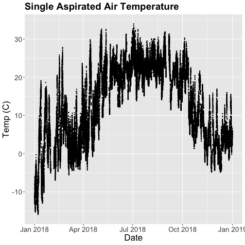
That looks better! But we're still working with the 30-minute data.
Aggregate Data by Day
We can use the dplyr package functions to aggregate the data. However, we have to choose which data we want to aggregate. Again, you might want daily minimum temps, mean temperature or maximum temps depending on your question.
In the context of phenology, minimum temperatures might be very important if you are interested in a species that is very frost susceptible. Any days with a minimum temperature below 0C could dramatically change the phenophase. For other species or meteorological zones, maximum thresholds may be very important. Or you might be mostinterested in the daily mean.
And note that you can combine different input values with different aggregation functions - for example, you could calculate the minimum of the half-hourly average temperature, or the average of the half-hourly maximum temperature.
For this tutorial, let's use maximum daily temperature, i.e. the maximum of the
tempSingleMax values for the day.
# convert to date, easier to work with
SAAT_30minC$Date <- as.Date(SAAT_30minC$startDateTime)
# max of mean temp each day
temp_day <- SAAT_30minC %>%
group_by(Date) %>%
distinct(Date, .keep_all=T) %>%
mutate(dayMax=max(tempSingleMaximum))
Now we can plot the cleaned up daily temperature.
# plot Air Temperature Data across 2018 using daily data
tempPlot_dayMax <- ggplot(temp_day, aes(Date, dayMax)) +
geom_point(size=0.5) +
ggtitle("Daily Max Air Temperature") +
xlab("") + ylab("Temp (C)") +
theme(plot.title = element_text(lineheight=.8, face="bold", size = 20)) +
theme(text = element_text(size=18))
tempPlot_dayMax
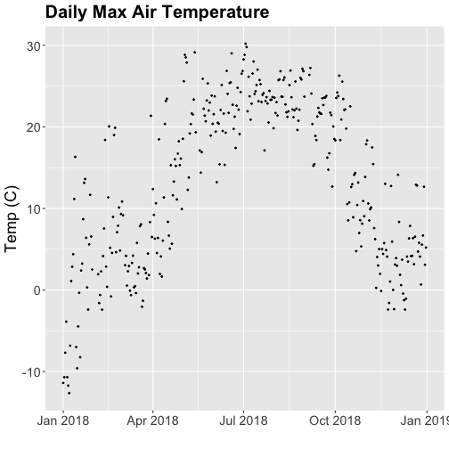
Thought questions:
- What do we gain by this visualization?
- What do we lose relative to the 30 minute intervals?
ggplot - Subset by Time
Sometimes we want to scale the x- or y-axis to a particular time subset without
subsetting the entire data_frame. To do this, we can define start and end
times. We can then define these limits in the scale_x_date object as
follows:
scale_x_date(limits=start.end) +
Let's plot just the first three months of the year.
# Define Start and end times for the subset as R objects that are the time class
startTime <- as.Date("2018-01-01")
endTime <- as.Date("2018-03-31")
# create a start and end time R object
start.end <- c(startTime,endTime)
str(start.end)
## Date[1:2], format: "2018-01-01" "2018-03-31"
# View data for first 3 months only
# And we'll add some color for a change.
tempPlot_dayMax3m <- ggplot(temp_day, aes(Date, dayMax)) +
geom_point(color="blue", size=0.5) +
ggtitle("Air Temperature\n Jan - March") +
xlab("Date") + ylab("Air Temperature (C)")+
(scale_x_date(limits=start.end,
date_breaks="1 week",
date_labels="%b %d"))
tempPlot_dayMax3m
## Warning: Removed 268 rows containing missing values (`geom_point()`).
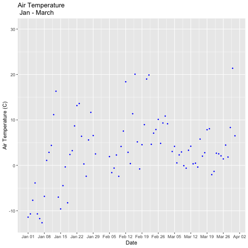
Now we have the temperature data matching our Phenology data from the previous tutorial, we want to save it to our computer to use in future analyses (or the next tutorial). This is optional if you are continuing directly to the next tutorial as you already have the data in R.
# Write .csv - this step is optional
# This will write to the working directory we set at the start of the tutorial
write.csv(temp_day , file="NEONsaat_daily_SCBI_2018.csv", row.names=F)
Get Lesson Code
Plot Continuous & Discrete Data Together
Last Updated: Apr 2, 2026
This tutorial discusses ways to plot plant phenology (discrete time series) and single-aspirated temperature (continuous time series) together. It uses data frames created in the first two parts of this series, Work with NEON OS & IS Data - Plant Phenology & Temperature. If you have not completed these tutorials, please download the dataset below.
Objectives
After completing this tutorial, you will be able to:
- plot multiple figures together with grid.arrange()
- plot only a subset of dates
Things You’ll Need To Complete This Tutorial
You will need the most current version of R and, preferably, RStudio loaded
on your computer to complete this tutorial.
Install R Packages
-
neonUtilities:
install.packages("neonUtilities") -
ggplot2:
install.packages("ggplot2") -
dplyr:
install.packages("dplyr") -
gridExtra:
install.packages("gridExtra")
More on Packages in R – Adapted from Software Carpentry.
Download Data
This tutorial is designed to have you download data directly from the NEON
portal API using the neonUtilities package. However, you can also directly
download this data, prepackaged, from FigShare. This data set includes all the
files needed for the Work with NEON OS & IS Data - Plant Phenology & Temperature
tutorial series. The data are in the format you would receive if downloading them
using the zipsByProduct() function in the neonUtilities package.
To start, we need to set up our R environment. If you're continuing from the previous tutorial in this series, you'll only need to load the new packages.
# Install needed package (only uncomment & run if not already installed)
#install.packages("dplyr")
#install.packages("ggplot2")
#install.packages("scales")
# Load required libraries
library(ggplot2)
library(dplyr)
##
## Attaching package: 'dplyr'
## The following objects are masked from 'package:stats':
##
## filter, lag
## The following objects are masked from 'package:base':
##
## intersect, setdiff, setequal, union
library(gridExtra)
##
## Attaching package: 'gridExtra'
## The following object is masked from 'package:dplyr':
##
## combine
library(scales)
options(stringsAsFactors=F) #keep strings as character type not factors
# set working directory to ensure R can find the file we wish to import and where
# we want to save our files. Be sure to move the download into your working directory!
wd <- "~/Documents/data/" # Change this to match your local environment
setwd(wd)
If you don't already have the R objects, temp_day and phe_1sp_2018, loaded
you'll need to load and format those data. If you do, you can skip this code.
# Read in data -> if in series this is unnecessary
temp_day <- read.csv(paste0(wd,'NEON-pheno-temp-timeseries/NEONsaat_daily_SCBI_2018.csv'))
phe_1sp_2018 <- read.csv(paste0(wd,'NEON-pheno-temp-timeseries/NEONpheno_LITU_Leaves_SCBI_2018.csv'))
# Convert dates
temp_day$Date <- as.Date(temp_day$Date)
# use dateStat - the date the phenophase status was recorded
phe_1sp_2018$dateStat <- as.Date(phe_1sp_2018$dateStat)
Separate Plots, Same Panel
In this dataset, we have phenology and temperature data from the Smithsonian Conservation Biology Institute (SCBI) NEON field site. There are a variety of ways we may want to look at this data, including aggregated at the site level, by a single plot, or viewing all plots at the same time but in separate plots. In the Work With NEON's Plant Phenology Data and the Work with NEON's Single-Aspirated Air Temperature Data tutorials, we created separate plots of the number of individuals who had leaves at different times of the year and the temperature in 2018.
However, plot the data next to each other to aid comparisons. The grid.arrange()
function from the gridExtra package can help us do this.
# first, create one plot
phenoPlot <- ggplot(phe_1sp_2018, aes(dateStat, countYes)) +
geom_bar(stat="identity", na.rm = TRUE) +
ggtitle("Total Individuals in Leaf") +
xlab("") + ylab("Number of Individuals")
# create second plot of interest
tempPlot_dayMax <- ggplot(temp_day, aes(Date, dayMax)) +
geom_point() +
ggtitle("Daily Max Air Temperature") +
xlab("Date") + ylab("Temp (C)")
# Then arrange the plots - this can be done with >2 plots as well.
grid.arrange(phenoPlot, tempPlot_dayMax)
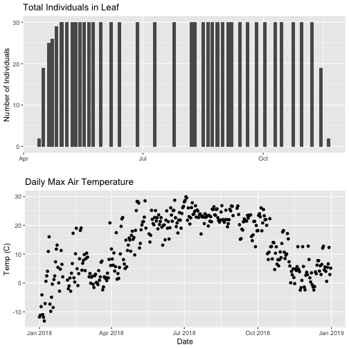
Now, we can see both plots in the same window. But, hmmm... the x-axis on both plots is kinda wonky. We want the same spacing in the scale across the year (e.g., July in one should line up with July in the other) plus we want the dates to display in the same format(e.g. 2016-07 vs. Jul vs Jul 2018).
Format Dates in Axis Labels
The date format parameter can be adjusted with scale_x_date. Let's format the x-axis
ticks so they read "month" (%b) in both graphs. We will use the syntax:
scale_x_date(labels=date_format("%b"")
Rather than re-coding the entire plot, we can add the scale_x_date element
to the plot object phenoPlot we just created.
-
You can type
?strptimeinto the R console to find a list of date format conversion specifications (e.g. %b = month). Typescale_x_datefor a list of parameters that allow you to format dates on the x-axis. -
If you are working with a date & time class (e.g. POSIXct), you can use
scale_x_datetimeinstead ofscale_x_date.
# format x-axis: dates
phenoPlot <- phenoPlot +
(scale_x_date(breaks = date_breaks("1 month"), labels = date_format("%b")))
tempPlot_dayMax <- tempPlot_dayMax +
(scale_x_date(breaks = date_breaks("1 month"), labels = date_format("%b")))
# New plot.
grid.arrange(phenoPlot, tempPlot_dayMax)
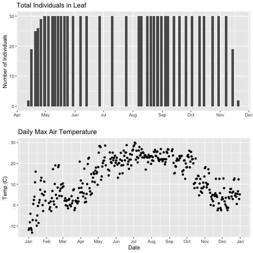
But this only solves one of the problems, we still have a different range on the x-axis which makes it harder to see trends.
Align data sets with different start dates
Now let's work to align the values on the x-axis. We can do this in two ways,
- setting the x-axis to have the same date range or 2) by filtering the dataset itself to only include the overlapping data. Depending on what you are trying to demonstrate and if you're doing additional analyses and want only the overlapping data, you may prefer one over the other. Let's try both.
Set range of x-axis
Alternatively, we can set the x-axis range for both plots by adding the limits
parameter to the scale_x_date() function.
# first, lets recreate the full plot and add in the
phenoPlot_setX <- ggplot(phe_1sp_2018, aes(dateStat, countYes)) +
geom_bar(stat="identity", na.rm = TRUE) +
ggtitle("Total Individuals in Leaf") +
xlab("") + ylab("Number of Individuals") +
scale_x_date(breaks = date_breaks("1 month"),
labels = date_format("%b"),
limits = as.Date(c('2018-01-01','2018-12-31')))
# create second plot of interest
tempPlot_dayMax_setX <- ggplot(temp_day, aes(Date, dayMax)) +
geom_point() +
ggtitle("Daily Max Air Temperature") +
xlab("Date") + ylab("Temp (C)") +
scale_x_date(date_breaks = "1 month",
labels=date_format("%b"),
limits = as.Date(c('2018-01-01','2018-12-31')))
# Plot
grid.arrange(phenoPlot_setX, tempPlot_dayMax_setX)
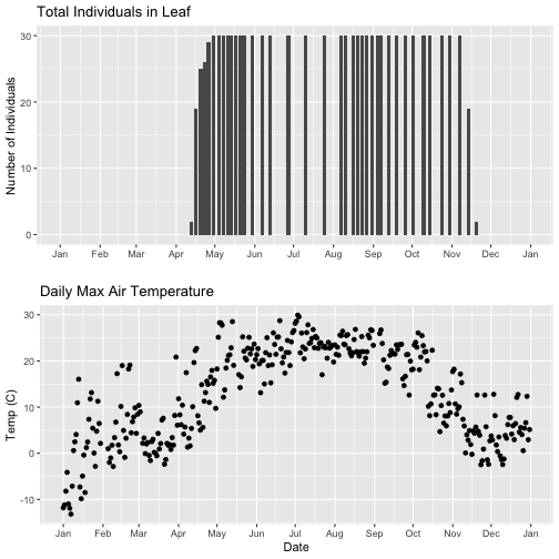
Now we can really see the pattern over the full year. This emphasizes the point that during much of the late fall, winter, and early spring none of the trees have leaves on them (or that data were not collected - this plot would not distinguish between the two).
Subset one data set to match other
Alternatively, we can simply filter the dataset with the larger date range so the we only plot the data from the overlapping dates.
# filter to only having overlapping data
temp_day_filt <- filter(temp_day, Date >= min(phe_1sp_2018$dateStat) &
Date <= max(phe_1sp_2018$dateStat))
# Check
range(phe_1sp_2018$date)
## [1] "2018-04-13" "2018-11-20"
range(temp_day_filt$Date)
## [1] "2018-04-13" "2018-11-20"
#plot again
tempPlot_dayMaxFiltered <- ggplot(temp_day_filt, aes(Date, dayMax)) +
geom_point() +
scale_x_date(breaks = date_breaks("months"), labels = date_format("%b")) +
ggtitle("Daily Max Air Temperature") +
xlab("Date") + ylab("Temp (C)")
grid.arrange(phenoPlot, tempPlot_dayMaxFiltered)
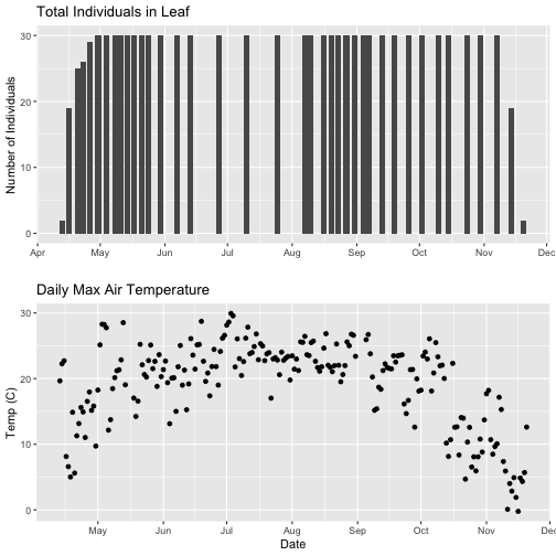
With this plot, we really look at the area of overlap in the plotted data (but this does cut out the time where the data are collected but not plotted).
Same plot with two Y-axes
What about layering these plots and having two y-axes (right and left) that have the different scale bars?
Some argue that you should not do this as it can distort what is actually going
on with the data. The author of the ggplot2 package is one of these individuals.
Therefore, you cannot use ggplot() to create a single plot with multiple y-axis
scales. You can read his own discussion of the topic on this
StackOverflow post.
However, individuals have found work arounds for these plots. The code below is provided as a demonstration of this capability. Note, by showing this code here, we don't necessarily endorse having plots with two y-axes.
This code is adapted from code by Jake Heare.
# Source: http://heareresearch.blogspot.com/2014/10/10-30-2014-dual-y-axis-graph-ggplot2_30.html
# Additional packages needed
library(gtable)
library(grid)
# Plot 1: Pheno data as bars, temp as scatter
grid.newpage()
phenoPlot_2 <- ggplot(phe_1sp_2018, aes(dateStat, countYes)) +
geom_bar(stat="identity", na.rm = TRUE) +
scale_x_date(breaks = date_breaks("1 month"), labels = date_format("%b")) +
ggtitle("Total Individuals in Leaf vs. Temp (C)") +
xlab(" ") + ylab("Number of Individuals") +
theme_bw()+
theme(legend.justification=c(0,1),
legend.position=c(0,1),
plot.title=element_text(size=25,vjust=1),
axis.text.x=element_text(size=20),
axis.text.y=element_text(size=20),
axis.title.x=element_text(size=20),
axis.title.y=element_text(size=20))
tempPlot_dayMax_corr_2 <- ggplot() +
geom_point(data = temp_day_filt, aes(Date, dayMax),color="red") +
scale_x_date(breaks = date_breaks("months"), labels = date_format("%b")) +
xlab("") + ylab("Temp (C)") +
theme_bw() %+replace%
theme(panel.background = element_rect(fill = NA),
panel.grid.major.x=element_blank(),
panel.grid.minor.x=element_blank(),
panel.grid.major.y=element_blank(),
panel.grid.minor.y=element_blank(),
axis.text.y=element_text(size=20,color="red"),
axis.title.y=element_text(size=20))
g1<-ggplot_gtable(ggplot_build(phenoPlot_2))
g2<-ggplot_gtable(ggplot_build(tempPlot_dayMax_corr_2))
pp<-c(subset(g1$layout,name=="panel",se=t:r))
g<-gtable_add_grob(g1, g2$grobs[[which(g2$layout$name=="panel")]],pp$t,pp$l,pp$b,pp$l)
ia<-which(g2$layout$name=="axis-l")
ga <- g2$grobs[[ia]]
ax <- ga$children[[2]]
ax$widths <- rev(ax$widths)
ax$grobs <- rev(ax$grobs)
ax$grobs[[1]]$x <- ax$grobs[[1]]$x - unit(1, "npc") + unit(0.15, "cm")
g <- gtable_add_cols(g, g2$widths[g2$layout[ia, ]$l], length(g$widths) - 1)
g <- gtable_add_grob(g, ax, pp$t, length(g$widths) - 1, pp$b)
grid.draw(g)
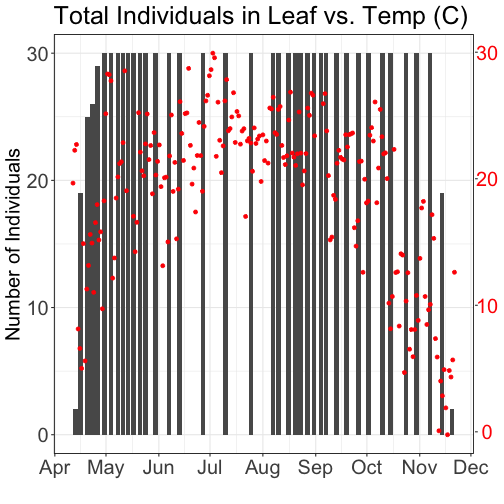
# Plot 2: Both pheno data and temp data as line graphs
grid.newpage()
phenoPlot_3 <- ggplot(phe_1sp_2018, aes(dateStat, countYes)) +
geom_line(na.rm = TRUE) +
scale_x_date(breaks = date_breaks("months"), labels = date_format("%b")) +
ggtitle("Total Individuals in Leaf vs. Temp (C)") +
xlab("Date") + ylab("Number of Individuals") +
theme_bw()+
theme(legend.justification=c(0,1),
legend.position=c(0,1),
plot.title=element_text(size=25,vjust=1),
axis.text.x=element_text(size=20),
axis.text.y=element_text(size=20),
axis.title.x=element_text(size=20),
axis.title.y=element_text(size=20))
tempPlot_dayMax_corr_3 <- ggplot() +
geom_line(data = temp_day_filt, aes(Date, dayMax),color="red") +
scale_x_date(breaks = date_breaks("months"), labels = date_format("%b")) +
xlab("") + ylab("Temp (C)") +
theme_bw() %+replace%
theme(panel.background = element_rect(fill = NA),
panel.grid.major.x=element_blank(),
panel.grid.minor.x=element_blank(),
panel.grid.major.y=element_blank(),
panel.grid.minor.y=element_blank(),
axis.text.y=element_text(size=20,color="red"),
axis.title.y=element_text(size=20))
g1<-ggplot_gtable(ggplot_build(phenoPlot_3))
g2<-ggplot_gtable(ggplot_build(tempPlot_dayMax_corr_3))
pp<-c(subset(g1$layout,name=="panel",se=t:r))
g<-gtable_add_grob(g1, g2$grobs[[which(g2$layout$name=="panel")]],pp$t,pp$l,pp$b,pp$l)
ia<-which(g2$layout$name=="axis-l")
ga <- g2$grobs[[ia]]
ax <- ga$children[[2]]
ax$widths <- rev(ax$widths)
ax$grobs <- rev(ax$grobs)
ax$grobs[[1]]$x <- ax$grobs[[1]]$x - unit(1, "npc") + unit(0.15, "cm")
g <- gtable_add_cols(g, g2$widths[g2$layout[ia, ]$l], length(g$widths) - 1)
g <- gtable_add_grob(g, ax, pp$t, length(g$widths) - 1, pp$b)
grid.draw(g)
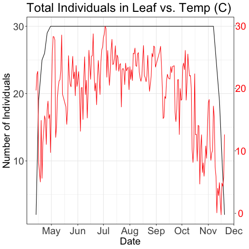
Get Lesson Code
Download and work with NEON Aquatic Instrument Data
Last Updated: Apr 2, 2026
This tutorial covers downloading NEON Aquatic Instrument System (AIS) data using the neonUtilities R package, as well as basic instruction in exploring and working with the downloaded data. You will learn how to navigate data documentation, separate data using the horizontalPosition variable, and interpret quality flags.
Objectives
After completing this activity, you will be able to:
- Download NEON AIS data using the
neonUtilitiespackage. - Understand how data sets are formatted and load them into R for analysis.
- Separate data collected at different sensor locations using the horizontalPosition variable.
- Understand and filter data using quality flags.
Things You'll Need To Complete This Tutorial
To complete this tutorial you will need R (version >4.1) and, preferably, RStudio loaded on your computer.
Install R Packages
- neonUtilities: Basic functions for accessing and working with NEON data
- ggplot2: Plotting functions
These packages are on CRAN and can be installed by
install.packages().
Additional Resources
Download Files and Load Directly to R: loadByProduct()
The most popular function in neonUtilities is loadByProduct().
This function downloads data from the NEON API, merges the site-by-month
files, and loads the resulting data tables into the R environment,
assigning each data type to the appropriate R class. This is a popular
choice because it ensures you're always working with the most up-to-date data,
and it ends with ready-to-use tables in R. However, if you use it in
a workflow you run repeatedly, keep in mind it will re-download the
data every time.
Before we get the NEON data, we need to install (if not already done) and load
the neonUtilities R package, as well as other packages we will use in the
analysis.
# Install neonUtilities package if you have not yet.
install.packages("neonUtilities")
install.packages("ggplot2")
# Set global option to NOT convert all character variables to factors
options(stringsAsFactors=F)
# Load required packages
library(neonUtilities)
library(ggplot2)
The inputs to loadByProduct() control which data to download and how
to manage the processing. The following are frequently used inputs:
-
dpID: the NEON data product ID, e.g. "DP1.20288.001" -
site: 4-letter NEON site code, e.g. "ARIK", or vector of of multiple sites, e.g. "c("MART","ARIK","BARC")". Defaults to "all", meaning all sites. -
startdateandenddate: start and end dates for period to be downloaded in the form YYYY-MM, e.g. "2017-06". Defaults to NA, meaning all available data. -
package: specifies either "basic" or "expanded" data package. Expanded data packages generally include additional information about data quality, such as individual quality flag test results. Not every NEON data product has an expanded package; if the expanded package is requested but there isn't one, the basic package will be downloaded. -
release: release version to be downloaded, e.g. "RELEASE-2023". To download the most recent release as well as provisional data (not yet QAQC'ed and included in a versioned release) use "current". -
savepath: the file path you want to download to; defaults to the working directory. -
check.size: T or F; should the function pause before downloading data and warn you about the size of your download? Defaults to T; if you are using this function within a script or batch process you will want to set this to F. -
token: this allows you to input your NEON API token to obtain faster downloads.
Learn more about NEON API tokens in the Using an API Token when Accessing NEON Data with neonUtilities tutorial.
There are additional inputs you can learn about in the Use the neonUtilities R Package to Access NEON Data tutorial.
The dpID is the data product identifier of the data you want to
download. The DPID can be found on the
Explore Data Products page.
It will be in the form DP#.#####.###. For this tutorial, we'll use NEON's most commonly downloaded AIS data products, Water quality.
- DP1.20288.001: Water quality
Now it's time to consider the NEON field site of interest. If not specified, the default will download a data product from all sites. The following are 4-letter site codes for NEON's 34 aquatics sites as of 2020:
- ARIK = Arikaree River CO
- BARC = Barco Lake FL
- BIGC = Upper Big Creek CA
- BLDE = Black Deer Creek WY
- BLUE = Blue River OK
- BLWA = Black Warrior River AL
- CARI = Caribou Creek AK
- COMO = Como Creek CO
- CRAM = Crampton Lake WI
- CUPE = Rio Cupeyes PR
- FLNT = Flint River GA
- GUIL = Rio Yahuecas PR
- HOPB = Lower Hop Brook MA
- KING = Kings Creek KS
- LECO = LeConte Creek TN
- LEWI = Lewis Run VA
- LIRO = Little Rock Lake WI
- MART = Martha Creek WA
- MAYF = Mayfield Creek AL
- MCDI = McDiffett Creek KS
- MCRA = McRae Creek OR
- OKSR = Oksrukuyik Creek AK
- POSE = Posey Creek VA
- PRIN = Pringle Creek TX
- PRLA = Prairie Lake ND
- PRPO = Prairie Pothole ND
- REDB = Red Butte Creek UT
- SUGG = Suggs Lake FL
- SYCA = Sycamore Creek AZ
- TECR = Teakettle Creek CA
- TOMB = Lower Tombigbee River AL
- TOOK = Toolik Lake AK
- WALK = Walker Branch TN
- WLOU = West St Louis Creek CO
In this exercise, we will use data from only one NEON field site, Pringle Creek, TX from February 2020. Because we want to examine individual quality flags we will download the expanded package. We want the most current release. Finally, since we are only downloading one site-month of data we do not need to check the file size, but for larger downloads this is advisable.
# download data of interest - Water Quality
waq <- loadByProduct(dpID="DP1.20288.001", site="PRIN",
startdate="2020-02", enddate="2020-02",
package="expanded", release="current",
check.size = F)
Files Associated with Downloads
The data we've downloaded comes as a list of objects.
# view all components of the list
names(waq)
## [1] "ais_maintenance" "ais_multisondeCleanCal" "categoricalCodes_20288" "citation_20288_RELEASE-2023" "issueLog_20288"
## [6] "readme_20288" "science_review_flags_20288" "sensor_positions_20288" "variables_20288" "waq_instantaneous"
We can see that there are multiple objects in the downloaded water quality data.
One dataframe of data (waq_instantaneous) and multiple metadata files.
If you'd like you can use the $ operator to assign an object from an item in
the list. If you prefer to extract each table from the list and work with it as
independent objects, which we will do, you can use the list2env() function.
# unlist the variables and add to the global environment
list2env(waq, .GlobalEnv)
So what exactly are these files and why would you want to use them?
- data file(s): There will always be one or more dataframes that include the primary data of the data product you downloaded. Multiple dataframes are available when there are related datatables for a single data product. For example, some data products are averaged at multiple intervals (e.x. 5-min averages and 30-min averages).
- sensor_postions_#####: this file contains information about the coordinates of each sensor, relative to a reference location.
- variables_#####: this file contains all the variables found in the associated data table(s). This includes full definitions, units, and other important information.
- readme_#####: The readme file, with the corresponding 5 digits from the data product number, provides you with important information relevant to the data product.
- maintenance record(s): Some data products come with maintenance records with information related to cleaning and calibration of sensors.
Let's take a look at a couple of these.
# which sensor locations exist in the water quality dataset we just downloaded?
View(waq_instantaneous)
View(sensor_positions_20288)
View(variables_20288)
Data versioning and citation
Let's check what release(s) our data is from (remember we used "current"). Each static data release has a unique DOI that should be cited. If any provisional data is included it should also be cited (including download date), and archived because provisional data is non-static.
# which release is the data from?
unique(waq_instantaneous$release)
## [1] "RELEASE-2023"
Learn more about data versioning and appropriately reuse of NEON data on the NEON Data Guidelines and Policy page.
Data from Different Sensor Locations
NEON often collects the same type of data from sensors in different locations.
These data are delivered together but you will frequently want to plot the data
separately or only include data from one sensor in your analysis. NEON uses the
horizontalPosition variable in the data tables to describe which sensor
data is collected from. The horizontalPosition (HOR) is always a three digit
number. Non-shoreline HOR examples as of 2024 at AIS sites include:
- 101: stream sensors located at the upstream station on a monopod mount,
- 111: stream sensors located at the upstream station on an overhead cable mount,
- 131: stream sensors located at the upstream station on a stand alone pressure transducer mount,
- 102: stream sensors located at the downstream station on a monopod mount,
- 112: stream sensors located at the downstream station on an overhead cable mount
- 132: stream sensors located at the downstream station on a stand alone pressure transducer mount,
- 110: stream pressure transducers mounted directly to a staff gauge.
- 103: sensors mounted on buoys in lakes or rivers
- 130, 140, 150, 160, 180 and and 190: sensors mounted in the littoral zone of lakes
Note that data is also collected at different vertical positions (VER) at lake and river sites. This example is from a wadeable stream site with only a single VER.
You'll frequently want to know which sensor locations are represented in your
data. We can do this by looking for the unique() position designations in
horizontalPostions.
# which sensor locations exist in the water quality dataset we just downloaded?
unique(waq_instantaneous$horizontalPosition)
## [1] "101" "102"
We can see that there are two water quality horizontal positions present in the data, upstream and downstream. As the HOR of sensors can change at sites over time, as well as the physical location corresponding to a particular HOR, it is a good idea to review the sensor_positions file when you're adding in new sites or a new date range to your analyses.
We can use this information to split water quality data into the two different sensor set locations: upstream and the downstream.
# Split data into separate dataframes by upstream/downstream locations.
waq_up <-
waq_instantaneous[(waq_instantaneous$horizontalPosition=="101"),]
waq_down <-
waq_instantaneous[(waq_instantaneous$horizontalPosition=="102"),]
Plot Data
Now that we have our data separated into the upstream and downstream data, let's plot Dissolved Oxygen from the downstream sensor. NEON also includes uncertainty estimates for most of its measurements. Let's include those in the plot as well.
First, let's identify the column names important for plotting - time and dissolved oxygen data:
# One option is to view column names in the data frame
colnames(waq_instantaneous)
## [1] "domainID" "siteID" "horizontalPosition" "verticalPosition"
## [5] "startDateTime" "endDateTime" "sensorDepth" "sensorDepthExpUncert"
## [9] "sensorDepthRangeQF" "sensorDepthNullQF" "sensorDepthGapQF" "sensorDepthValidCalQF"
## [13] "sensorDepthSuspectCalQF" "sensorDepthPersistQF" "sensorDepthAlphaQF" "sensorDepthBetaQF"
## [17] "sensorDepthFinalQF" "sensorDepthFinalQFSciRvw" "specificConductance" "specificConductanceExpUncert"
## [21] "specificConductanceRangeQF" "specificConductanceStepQF" "specificConductanceNullQF" "specificConductanceGapQF"
## [25] "specificConductanceSpikeQF" "specificConductanceValidCalQF" "specificCondSuspectCalQF" "specificConductancePersistQF"
## [29] "specificConductanceAlphaQF" "specificConductanceBetaQF" "specificCondFinalQF" "specificCondFinalQFSciRvw"
## [33] "dissolvedOxygen" "dissolvedOxygenExpUncert" "dissolvedOxygenRangeQF" "dissolvedOxygenStepQF"
## [37] "dissolvedOxygenNullQF" "dissolvedOxygenGapQF" "dissolvedOxygenSpikeQF" "dissolvedOxygenValidCalQF"
## [41] "dissolvedOxygenSuspectCalQF" "dissolvedOxygenPersistenceQF" "dissolvedOxygenAlphaQF" "dissolvedOxygenBetaQF"
## [45] "dissolvedOxygenFinalQF" "dissolvedOxygenFinalQFSciRvw" "seaLevelDissolvedOxygenSat" "seaLevelDOSatExpUncert"
## [49] "seaLevelDOSatRangeQF" "seaLevelDOSatStepQF" "seaLevelDOSatNullQF" "seaLevelDOSatGapQF"
## [53] "seaLevelDOSatSpikeQF" "seaLevelDOSatValidCalQF" "seaLevelDOSatSuspectCalQF" "seaLevelDOSatPersistQF"
## [57] "seaLevelDOSatAlphaQF" "seaLevelDOSatBetaQF" "seaLevelDOSatFinalQF" "seaLevelDOSatFinalQFSciRvw"
## [61] "localDissolvedOxygenSat" "localDOSatExpUncert" "localDOSatRangeQF" "localDOSatStepQF"
## [65] "localDOSatNullQF" "localDOSatGapQF" "localDOSatSpikeQF" "localDOSatValidCalQF"
## [69] "localDOSatSuspectCalQF" "localDOSatPersistQF" "localDOSatAlphaQF" "localDOSatBetaQF"
## [73] "localDOSatFinalQF" "localDOSatFinalQFSciRvw" "pH" "pHExpUncert"
## [77] "pHRangeQF" "pHStepQF" "pHNullQF" "pHGapQF"
## [81] "pHSpikeQF" "pHValidCalQF" "pHSuspectCalQF" "pHPersistenceQF"
## [85] "pHAlphaQF" "pHBetaQF" "pHFinalQF" "pHFinalQFSciRvw"
## [89] "chlorophyll" "chlorophyllExpUncert" "chlorophyllRangeQF" "chlorophyllStepQF"
## [93] "chlorophyllNullQF" "chlorophyllGapQF" "chlorophyllSpikeQF" "chlorophyllValidCalQF"
## [97] "chlorophyllSuspectCalQF" "chlorophyllPersistenceQF" "chlorophyllAlphaQF" "chlorophyllBetaQF"
## [101] "chlorophyllFinalQF" "chlorophyllFinalQFSciRvw" "chlaRelativeFluorescence" "chlaRelFluoroExpUncert"
## [105] "chlaRelFluoroRangeQF" "chlaRelFluoroStepQF" "chlaRelFluoroNullQF" "chlaRelFluoroGapQF"
## [109] "chlaRelFluoroSpikeQF" "chlaRelFluoroValidCalQF" "chlaRelFluoroSuspectCalQF" "chlaRelFluoroPersistenceQF"
## [113] "chlaRelFluoroAlphaQF" "chlaRelFluoroBetaQF" "chlaRelFluoroFinalQF" "chlaRelFluoroFinalQFSciRvw"
## [117] "turbidity" "turbidityExpUncert" "turbidityRangeQF" "turbidityStepQF"
## [121] "turbidityNullQF" "turbidityGapQF" "turbiditySpikeQF" "turbidityValidCalQF"
## [125] "turbiditySuspectCalQF" "turbidityPersistenceQF" "turbidityAlphaQF" "turbidityBetaQF"
## [129] "turbidityFinalQF" "turbidityFinalQFSciRvw" "fDOM" "rawCalibratedfDOM"
## [133] "fDOMExpUncert" "fDOMRangeQF" "fDOMStepQF" "fDOMNullQF"
## [137] "fDOMGapQF" "fDOMSpikeQF" "fDOMValidCalQF" "fDOMSuspectCalQF"
## [141] "fDOMPersistenceQF" "fDOMAlphaQF" "fDOMBetaQF" "fDOMTempQF"
## [145] "fDOMAbsQF" "fDOMFinalQF" "fDOMFinalQFSciRvw" "buoyNAFlag"
## [149] "spectrumCount" "publicationDate" "release"
# Alternatively, view the variables object corresponding to the data product for more information
View(variables_20288)
Quite a few columns in the water quality data product!
The time column we'll consider for instrumented systems is endDateTime.
Timestamp column choice (e.g. start or end) matters for time-aggregated
datasets, but should not matter for instantaneous data such as water quality.
When interpreting data, keep in mind NEON timestamps are always in UTC.
The data columns we would like to plot are dissolvedOxygen and
dissolvedOxygenExpUncert.
# plot
doPlot <- ggplot() +
geom_line(data = waq_down,aes(endDateTime, dissolvedOxygen),na.rm=TRUE, color="blue") +
geom_ribbon(data=waq_down,aes(x=endDateTime,
ymin = (dissolvedOxygen - dissolvedOxygenExpUncert),
ymax = (dissolvedOxygen + dissolvedOxygenExpUncert)),
alpha = 0.4, fill = "grey25") +
ylim(8, 15) + ylab("DO (mg/L)") + xlab("Date") + ggtitle("PRIN Downstream DO with Uncertainty Bounds")
doPlot
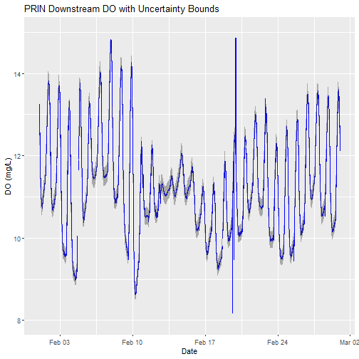
Examine Quality Flagged Data
Data product quality flags fall under two distinct types:
- Automated quality flags, e.g. range, spike, step, null
- Manual science review quality flag
In instantaneous data such as water quality, the quality flag columns are denoted with "QF". In time-averaged data, most quality flags have been aggregated into quality metrics, with column names denoted with "QM" representing the fraction of flagged points within the time averaging window.
waq_qf_names <- names(waq_down)[grep("QF", names(waq_down))]
print(paste0("Total columns in DP1.20288.001 expanded package = ",
as.character(length(waq_qf_names))))
## [1] "Total columns in DP1.20288.001 expanded package = 120"
# Let's just look at those corresponding to dissolvedOxygen.
# We need to remove those associated with dissolvedOxygenSaturation.
do_qf_names <- waq_qf_names[grep("dissolvedOxygen",waq_qf_names)]
do_qf_names <- do_qf_names[grep("dissolvedOxygenSat",do_qf_names,invert=T)]
print("dissolvedOxygen columns in DP1.20288.001 expanded package:")
## [1] "dissolvedOxygen columns in DP1.20288.001 expanded package:"
print(do_qf_names)
## [1] "dissolvedOxygenRangeQF" "dissolvedOxygenStepQF" "dissolvedOxygenNullQF" "dissolvedOxygenGapQF"
## [5] "dissolvedOxygenSpikeQF" "dissolvedOxygenValidCalQF" "dissolvedOxygenSuspectCalQF" "dissolvedOxygenPersistenceQF"
## [9] "dissolvedOxygenAlphaQF" "dissolvedOxygenBetaQF" "dissolvedOxygenFinalQF" "dissolvedOxygenFinalQFSciRvw"
A quality flag (QF) of 0 indicates a pass, 1 indicates a fail, and -1 indicates a test that could not be performed. For example, a range test cannot be performed on missing measurements.
Detailed quality flags test results are all available in the
package = 'expanded' setting we specified when calling
neonUtilities::loadByProduct(). If we had specified package = 'basic',
we wouldn't be able to investigate the detail in the type of data flag thrown.
We would only see the FinalQF columns.
The AlphaQF and BetaQF represent aggregated results of various QF tests,
and vary by a data product's algorithm. In most cases, an observation's
AlphaQF = 1 indicates whether or not at least one QF was set to a value
of 1, and an observation's BetaQF = 1 indicates whether or not at least one
QF was set to value of -1.
Let's consider what types of quality flags were thrown.
for(col_nam in do_qf_names){
print(paste0(col_nam, " unique values: ",
paste0(unique(waq_down[,col_nam]),
collapse = ", ")))
}
## [1] "dissolvedOxygenRangeQF unique values: 0, -1"
## [1] "dissolvedOxygenStepQF unique values: 0, -1, 1"
## [1] "dissolvedOxygenNullQF unique values: 0, 1"
## [1] "dissolvedOxygenGapQF unique values: 0, 1"
## [1] "dissolvedOxygenSpikeQF unique values: 0, -1"
## [1] "dissolvedOxygenValidCalQF unique values: 0"
## [1] "dissolvedOxygenSuspectCalQF unique values: 0"
## [1] "dissolvedOxygenPersistenceQF unique values: 0"
## [1] "dissolvedOxygenAlphaQF unique values: 0, 1"
## [1] "dissolvedOxygenBetaQF unique values: 0, 1"
## [1] "dissolvedOxygenFinalQF unique values: 0, 1"
## [1] "dissolvedOxygenFinalQFSciRvw unique values: NA"
QF values generally mean the following:
- 0: Quality test passed
- 1: Quality test failed
- -1: Quality test could not be run
Now let's consider the total number of flags generated for each quality test:
# Loop across the QF column names.
# Within each column, count the number of rows that equal '1'.
print("FLAG TEST - COUNT")
## [1] "FLAG TEST - COUNT"
for (col_nam in do_qf_names){
totl_qf_in_col <- length(which(waq_down[,col_nam] == 1))
print(paste0(col_nam,": ",totl_qf_in_col))
}
## [1] "dissolvedOxygenRangeQF: 0"
## [1] "dissolvedOxygenStepQF: 23"
## [1] "dissolvedOxygenNullQF: 224"
## [1] "dissolvedOxygenGapQF: 211"
## [1] "dissolvedOxygenSpikeQF: 0"
## [1] "dissolvedOxygenValidCalQF: 0"
## [1] "dissolvedOxygenSuspectCalQF: 0"
## [1] "dissolvedOxygenPersistenceQF: 0"
## [1] "dissolvedOxygenAlphaQF: 247"
## [1] "dissolvedOxygenBetaQF: 229"
## [1] "dissolvedOxygenFinalQF: 247"
## [1] "dissolvedOxygenFinalQFSciRvw: 0"
print(paste0("Total DO observations: ", nrow(waq_down) ))
## [1] "Total DO observations: 41760"
Above lists the total DO QFs, as well as the total number of observation data points in the data file.
For specific details on the algorithms used to create a data product and its corresponding quality tests, it's best to first check the data product's Algorithm Theoretical Basis Document (ATBD) available for download on the data product's web page.
Are there any manual science review quality flags? If so, the explanation for flagging may also be viewed science_review_flags file that comes with the download.
Note that the automated quality flag algorithms are not perfect, and suspect data points may occasionally pass the quality tests. Other times potentially useful data may get quality flagged. Ultimately it is up to the user to decide which data they are comfortable using, which is why we recommend using the expanded data package to better understand why data are being flagged.
Replot, with quality flags filtered by color
Let's replot the data with any quality flagged measurements set to a different color.
# plot
doPlot <- ggplot() +
geom_line(data = waq_down, aes(x=endDateTime, y=dissolvedOxygen,
color=factor(dissolvedOxygenFinalQF)), na.rm=TRUE) +
scale_color_manual(values = c("0" = "blue","1"="red")) +
ylim(8, 15) + ylab("DO (mg/L)") + xlab("Date") + ggtitle("PRIN Downstream DO filtered by FinalQF")
doPlot
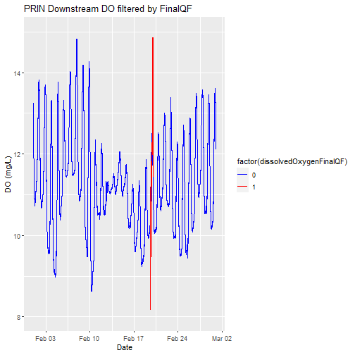
Apply what we've learned Part 1 - Temperature of Surface Water
Applying what we've learned, let's look at a different data product,Temperature of Surface Water (DP1.20053.001). Can you download for the same site and month that we just looked at for water quality?
# download continuous discharge data
csd <- loadByProduct(dpID="DP1.20053.001", site="PRIN",
startdate="2020-02", enddate="2020-02",
package="expanded", release="current",
check.size = F)
list2env(csd,.GlobalEnv)
This data product also comes with sensor_position_#####, variables_#####, readme_#####, and other metadata files. But did you notice anything different about the data file(s)? Temperature of surface water is an averaged data product and comes with both a 5min and 30min data file. Let's use the 30min.
What horizontal positions are present in the data?
# which sensor locations exist in the temperature of surface water dataset?
unique(TSW_30min$horizontalPosition)
## [1] "101" "102"
Let's use the downstream data just like we did for water quality.
# Split data into separate dataframe for downstream location.
tsw_down <-
TSW_30min[(TSW_30min$horizontalPosition=="102"),]
Can you remove the quality flagged values?
# remove values with a final quality flag
tsw_down<-tsw_down[(tsw_down$finalQF=="0"),]
Can you plot the data?
# plot
csdPlot <- ggplot() +
geom_line(data = tsw_down,aes(endDateTime, surfWaterTempMean),na.rm=TRUE, color="blue") +
geom_ribbon(data=tsw_down,aes(x=endDateTime,
ymin = (surfWaterTempMean-surfWaterTempExpUncert),
ymax = (surfWaterTempMean+surfWaterTempExpUncert)),
alpha = 0.4, fill = "grey25") +
ylim(2, 16) + ylab("Temp (C)") + xlab("Date") + ggtitle("PRIN Downstream Temp with Uncertainty Bounds")
csdPlot
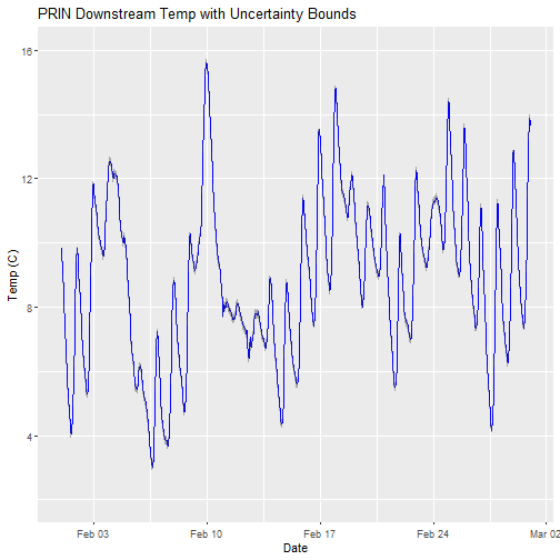
Apply what we've learned Part 2 - Continuous discharge
Applying what we've learned, let's look at a different data product, Continuous discharge (DP4.00130.001). Can you download for the same site and month that we just looked at for water quality?
# download continuous discharge data
csd <- loadByProduct(dpID="DP4.00130.001", site="PRIN",
startdate="2020-02", enddate="2020-02",
package="expanded", release="current",
check.size = F)
list2env(csd,.GlobalEnv)
Discharge is only measured a a single location in stream sites, so we don't have to worry about horizontal position. Can you remove the quality flagged values?
# remove values with a final quality flag
csd_continuousDischarge<-csd_continuousDischarge[(csd_continuousDischarge$dischargeFinalQF=="0"),]
Can you plot the discharge data?
# plot
csdPlot <- ggplot() +
geom_line(data = csd_continuousDischarge,aes(endDate, maxpostDischarge),na.rm=TRUE, color="blue") +
geom_ribbon(data=csd_continuousDischarge,aes(x=endDate,
ymin = (withRemnUncQLower1Std),
ymax = (withRemnUncQUpper1Std)),
alpha = 0.4, fill = "grey25") +
ylim(0, 4000) + ylab("Q (L/s)") + xlab("Date") + ggtitle("PRIN Discharge with Uncertainty Bounds")
csdPlot
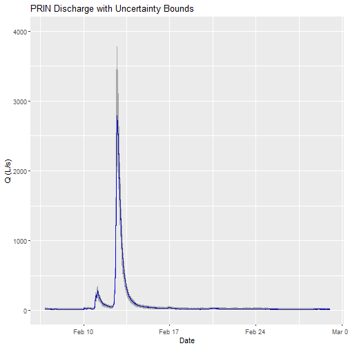
Note: The developers of the Bayesian discharge model used by NEON recommend the maxpostDischarge, which is the mode of the posterior distribution (means and medians are also provided).
Get Lesson Code
Using the neonOS Package to Check for Duplicates and Join Tables
Last Updated: Apr 2, 2026
NEON observational data are diverse in both content and in data structure. Generally, data are published in a set of data tables, each of which corresponds to a particular activity: for example, several data products include a field collection data table, a sample processing data table, and a table of laboratory analytical results.
Joining data tables
Depending on the analysis you want to carry out, there may be data in multiple tables that you want to bring together. For example, it is very common that species identifications are in a different table from chemical composition or pathogen status. For species-specific analyses, you would need to draw on multiple tables. There are a variety of ways to do this, but one of the simplest is to join the tables and create a single flat table.
The Quick Start Guides and Data Product User Guides provide information about the relationships between different data tables, and we recommend you consult these documents for the data products you are working with to gain the full picture. Quick Start Guides (QSGs) are included in the download package when you download data via the Data Portal, and can also be viewed on the Data Product Details page for each data product; for example, see the page for Plant foliar traits. Scroll down to the Documentation section to see the QSG. The Data Product User Guide is also available in the Documentation menu.
To join related tables, the neonOS package provides the
joinTableNEON() function, which checks the Table joining section of
the QSG, and uses the information there to join the tables if
possible. If the join isn't possible, or if it requires customized code,
the function will return an informative error, and usually refer you
to the QSG for more details.
Duplicates
One of the most common data entry errors that occurs in NEON OS data is
duplicate entry. NEON data entry applications and ingest validation rules
are designed to prevent duplicate entry where possible, but errors can't
be avoided completely. Consequently, NEON metadata for each OS data product
(the variables file) includes an indicator of which data fields, taken
together, should define a unique record. This combination of fields is
called the "primary key" for the data table. The neonOS function
removeDups() uses these metadata to identify duplicate records.
Depending on the content of the duplicate records, they may be resolved to
a single record or marked as unresolvable - see below for details.
In this tutorial, we will de-duplicate and then join two data tables in the Aquatic plant bryophyte chemical properties (DP1.20063.001) data product, using it as an example to demonstrate the operation of these two functions. Then we will take a look at Mosquitoes sampled from CO2 traps (DP1.10043.001), which contains more complicated table relationships, and see how to modify the code to work with those tables.
Objectives
After completing this activity, you will be able to:
- Identify and resolve duplicate data using the
neonOSpackage - Join NEON data tables using the
neonOSpackage
Things You’ll Need To Complete This Tutorial
You will need a version of R (4.0 or higher. This code may work with
earlier versions but it hasn't been tested) and, preferably, RStudio
loaded on your computer to complete this tutorial.
Install R Packages
-
neonUtilities:
install.packages("neonUtilities") -
neonOS:
install.packages("neonOS")
Additional Resources
- NEON Data Portal
- NEON Code Hub
Set Up R Environment and Download Data
First install and load the necessary packages.
# install packages. you can skip this step if
# the packages are already installed
install.packages("neonUtilities")
install.packages("neonOS")
install.packages("ggplot2")
# load packages
library(neonUtilities)
library(neonOS)
library(ggplot2)
We'll use aquatic plant chemistry (DP1.20063.001) as the example dataset. Use
the neonUtilities function loadByProduct() to download and read in the
data. If you're not familiar with the neonUtilities package and how to use
it to access NEON data, we recommend you follow the Download and Explore NEON Data
tutorial before proceeding with this one.
Here, we'll use the same subset of aquatic plant chemistry data as in the Download and Explore tutorial. Get the data from the Prairie Lake, Suggs Lake, and Toolik Lake sites, specifying the 2022 data release.
apchem <- loadByProduct(dpID="DP1.20063.001",
site=c("PRLA","SUGG","TOOK"),
package="expanded",
release="RELEASE-2022",
check.size=F)
Copy each of the downloaded tables into the R environment.
list2env(apchem, .GlobalEnv)
Identify and Resolve Duplicates
As noted above, duplicate data entry is a common error in human
data entry. removeDups() uses the definitional metadata in the
variables file to identify duplicates. It requires two inputs:
the data table, and the corresponding variables file.
apl_biomass <- removeDups(data=apl_biomass,
variables=variables_20063)
## No duplicated key values found!
There were no duplicates found in the apl_biomass data table.
A duplicateRecordQF quality flag has been added to the table,
and you can confirm that there were no duplicates by checking
the values of the flag.
unique(apl_biomass$duplicateRecordQF)
## [1] 0
All data have flag value = 0, indicating they are not duplicated.
Let's check the apl_plantExternalLabDataPerSample table.
apl_plantExternalLabDataPerSample <- removeDups(
data=apl_plantExternalLabDataPerSample,
variables=variables_20063)
10 duplicated key values found, representing 20 non-unique records. Attempting to resolve.
|==========================================================================================| 100%
2 resolveable duplicates merged into matching records
2 resolved records flagged with duplicateRecordQF=1
16 unresolveable duplicates flagged with duplicateRecordQF=2
The function output tells you there were 20 duplicates (out of 26108
total data records). Four of those duplicates were resolved, leaving two
records flagged as resolved duplicates, with duplicateRecordQF=1. The
remaining 16 couldn't be resolved, and were flagged with
duplicateRecordQF=2.
What does it mean for duplicates to be resolved? Some duplicates represent
identical data that have been entered multiple times, whereas some duplicates
have the same values in the primary key, but differ in data values.
removeDups() has a fairly narrow set of criteria for resolving to a single
record:
- If one data record has empty fields that are populated in the other record, the non-empty values are retained.
- If records are identical except for uid, remarks, and/or personnel (
identifiedBy,recordedBy, etc) fields, unique values are concatenated within the non-matching fields, separated by|(pipes).
Records that can be merged to a single record by these criteria are flagged
with duplicateRecordQF=1. Records with mis-matched data that can't be merged
are retained as-is and flagged with duplicateRecordQF=2.
Note that even in fully identical duplicates, the uid field (universal
identifier) will always be unique. Thus the uid field in merged records
will always contain the pipe-delimited set of uids of the original records.
What does this look like in practice? Let's look at the two resolved duplicates:
apl_plantExternalLabDataPerSample[which(
apl_plantExternalLabDataPerSample$duplicateRecordQF==1),]
## uid domainID siteID
## 55 cca9850e-165d-4cb7-9872-eff490c79ffa|1f5a5389-c18c-4fbf-81d6-9cd45e65f48a D03 SUGG
## 60 e6cab47f-427b-47a9-a281-cbfe7c101fc3|368e16bb-23d4-4596-b624-b338777bc9bc D03 SUGG
## namedLocation collectDate sampleID sampleCondition
## 55 SUGG.AOS.reach 2016-02-22 SUGG.20160222.UTFO.Q5 condition ok
## 60 SUGG.AOS.reach 2016-02-22 SUGG.20160222.UTFO.Q5 condition ok
## laboratoryName analysisDate analyzedBy sampleType replicate
## 55 Academy of Natural Sciences of Drexel University 2016-07-12 OKgcKejxXbI= CN 1
## 60 Academy of Natural Sciences of Drexel University 2016-07-12 OKgcKejxXbI= CN 1
## sampleVolumeFiltered filterSize percentFilterAnalyzed analyte analyteConcentration plantAlgaeLabUnits
## 55 NA 25 100 carbon 34.01 percent
## 60 NA 25 100 nitrogen 2.84 percent
## method externalRemarks publicationDate release duplicateRecordQF
## 55 <NA> <NA> 20211221T225348Z RELEASE-2022 1
## 60 <NA> <NA> 20211221T225348Z RELEASE-2022 1
You can see that both records have two pipe-delimited uids, and are flagged.
Let's look at the unresolveable duplicates:
apl_plantExternalLabDataPerSample[which(
apl_plantExternalLabDataPerSample$duplicateRecordQF==2),]
## uid domainID siteID namedLocation collectDate sampleID
## 1 5fa69a8b-d19e-40f1-84a8-e46ed08cdc59 D03 SUGG SUGG.AOS.reach 2014-07-09 SUGG.20140709.LISP2.1
## 2 cebefd95-f4c7-4e60-9b79-93efd3f27691 D03 SUGG SUGG.AOS.reach 2014-07-09 SUGG.20140709.LISP2.3
## 3 a4b6d931-b093-419e-bb69-0b684219405e D03 SUGG SUGG.AOS.reach 2014-07-09 SUGG.20140709.LISP2.1
## 4 f462390b-2d4a-4aec-92e1-b46a740ec40d D03 SUGG SUGG.AOS.reach 2014-07-09 SUGG.20140709.NULU.7
## 5 d4fa7f65-6b2b-46fa-9bca-529745970c56 D03 SUGG SUGG.AOS.reach 2014-07-09 SUGG.20140709.NULU.7
## 6 ab43c466-b235-4f3d-9146-a1f81a91012d D03 SUGG SUGG.AOS.reach 2014-07-09 SUGG.20140709.LISP2.3
## 7 1140a4c2-139e-40dc-a14d-c2446e3a5664 D03 SUGG SUGG.AOS.reach 2014-07-09 SUGG.20140709.NULU.9
## 8 5201dc04-da3d-4bc2-b2bf-668ad4a3ddb5 D03 SUGG SUGG.AOS.reach 2014-07-09 SUGG.20140709.NULU.7
## 9 1e36cdeb-4e94-431d-8342-5ce5ff6ac6ae D03 SUGG SUGG.AOS.reach 2014-07-09 SUGG.20140709.NULU.9
## 10 b98069a4-74fb-40d8-8b98-7a5aedea7912 D03 SUGG SUGG.AOS.reach 2014-07-09 SUGG.20140709.NULU.9
## 11 9633d367-bd10-4588-a6e2-cbe954327bf6 D03 SUGG SUGG.AOS.reach 2014-07-09 SUGG.20140709.NULU.9
## 12 309ccbe3-d4a8-4bd3-b773-85aa98dd7627 D03 SUGG SUGG.AOS.reach 2014-07-09 SUGG.20140709.LISP2.1
## 13 6d6b1da2-049f-439c-81c9-add482f6fab8 D03 SUGG SUGG.AOS.reach 2014-07-09 SUGG.20140709.LISP2.1
## 14 841e51f4-dcc9-45fc-937b-871678ff16f2 D03 SUGG SUGG.AOS.reach 2014-07-09 SUGG.20140709.LISP2.3
## 15 3e04c3a1-7e2f-4349-a1c2-822d736fc2cf D03 SUGG SUGG.AOS.reach 2014-07-09 SUGG.20140709.NULU.7
## 16 431a4418-fdd0-4566-8791-d16ecfce76eb D03 SUGG SUGG.AOS.reach 2014-07-09 SUGG.20140709.LISP2.3
## sampleCondition laboratoryName analysisDate analyzedBy sampleType
## 1 condition ok Academy of Natural Sciences of Drexel University 2015-02-05 OKgcKejxXbI= CN
## 2 condition ok Academy of Natural Sciences of Drexel University 2015-02-05 OKgcKejxXbI= CN
## 3 condition ok Academy of Natural Sciences of Drexel University 2015-02-05 OKgcKejxXbI= CN
## 4 condition ok Academy of Natural Sciences of Drexel University 2015-02-05 OKgcKejxXbI= CN
## 5 condition ok Academy of Natural Sciences of Drexel University 2015-02-05 OKgcKejxXbI= CN
## 6 condition ok Academy of Natural Sciences of Drexel University 2015-02-05 OKgcKejxXbI= CN
## 7 condition ok Academy of Natural Sciences of Drexel University 2015-02-05 OKgcKejxXbI= CN
## 8 condition ok Academy of Natural Sciences of Drexel University 2015-02-05 OKgcKejxXbI= CN
## 9 condition ok Academy of Natural Sciences of Drexel University 2015-02-05 OKgcKejxXbI= CN
## 10 condition ok Academy of Natural Sciences of Drexel University 2015-02-05 OKgcKejxXbI= CN
## 11 condition ok Academy of Natural Sciences of Drexel University 2015-02-05 OKgcKejxXbI= CN
## 12 condition ok Academy of Natural Sciences of Drexel University 2015-02-05 OKgcKejxXbI= CN
## 13 condition ok Academy of Natural Sciences of Drexel University 2015-02-05 OKgcKejxXbI= CN
## 14 condition ok Academy of Natural Sciences of Drexel University 2015-02-05 OKgcKejxXbI= CN
## 15 condition ok Academy of Natural Sciences of Drexel University 2015-02-05 OKgcKejxXbI= CN
## 16 condition ok Academy of Natural Sciences of Drexel University 2015-02-05 OKgcKejxXbI= CN
## replicate sampleVolumeFiltered filterSize percentFilterAnalyzed analyte analyteConcentration
## 1 1 NA 25 100 carbon 38.22
## 2 1 NA 25 100 nitrogen 2.26
## 3 1 NA 25 100 nitrogen 1.98
## 4 1 NA 25 100 carbon 43.79
## 5 1 NA 25 100 nitrogen 3.16
## 6 1 NA 25 100 carbon 39.77
## 7 1 NA 25 100 carbon 43.26
## 8 1 NA 25 100 nitrogen 3.14
## 9 1 NA 25 100 nitrogen 2.94
## 10 1 NA 25 100 carbon 43.20
## 11 1 NA 25 100 nitrogen 3.00
## 12 1 NA 25 100 carbon 38.23
## 13 1 NA 25 100 nitrogen 2.02
## 14 1 NA 25 100 nitrogen 2.23
## 15 1 NA 25 100 carbon 43.93
## 16 1 NA 25 100 carbon 39.66
## plantAlgaeLabUnits method externalRemarks publicationDate release duplicateRecordQF
## 1 percent <NA> Limnobium spongia 20220110T211020Z RELEASE-2022 2
## 2 percent <NA> Limnobium spongia 20220110T211020Z RELEASE-2022 2
## 3 percent <NA> Limnobium spongia 20220110T211020Z RELEASE-2022 2
## 4 percent <NA> Nuphar Luteum 20220110T211020Z RELEASE-2022 2
## 5 percent <NA> Nuphar Luteum 20220110T211020Z RELEASE-2022 2
## 6 percent <NA> Limnobium spongia 20220110T211020Z RELEASE-2022 2
## 7 percent <NA> Nuphar Luteum 20220110T211020Z RELEASE-2022 2
## 8 percent <NA> Nuphar Luteum 20220110T211020Z RELEASE-2022 2
## 9 percent <NA> Nuphar Luteum 20220110T211020Z RELEASE-2022 2
## 10 percent <NA> Nuphar Luteum 20220110T211020Z RELEASE-2022 2
## 11 percent <NA> Nuphar Luteum 20220110T211020Z RELEASE-2022 2
## 12 percent <NA> Limnobium spongia 20220110T211020Z RELEASE-2022 2
## 13 percent <NA> Limnobium spongia 20220110T211020Z RELEASE-2022 2
## 14 percent <NA> Limnobium spongia 20220110T211020Z RELEASE-2022 2
## 15 percent <NA> Nuphar Luteum 20220110T211020Z RELEASE-2022 2
## 16 percent <NA> Limnobium spongia 20220110T211020Z RELEASE-2022 2
The key for this data table is the sample identifier and analyte, and here there are multiple records with the same sample identifier, both for carbon and nitrogen values. The most likely scenario is that these are unlabeled replicate analyses, i.e., the lab ran multiple analyses on the same samples for quality control purposes, but forgot to label them accordingly.
Now, how should you proceed with your analysis? Of course, that is up to
you, and depends on your analysis. Because these appear to be unlabeled
analytical replicates, I would probably average the analyte values, but
a decision like this can't be made automatically - removeDups() can
identify the records of concern, but what to do with them is a
judgement call.
Of course, NEON scientists also review NEON data and identify duplicates as part of quality assurance and quality control procedures, and resolve them if possible. In the data download step above, we accessed RELEASE-2022. The data release is stable and reproducible over time, but duplicates you find in one release may be resolved in future releases.
Join Data Tables
If you are using neonOS to check for duplicates and also to join data
tables, the duplicate step should always come first. Because duplicate
identification uses the variables file to determine uniqueness of data
records, the duplicate check step requires that the data match the
variables file exactly, which they won't after being joined.
To join the apl_biomass and apl_plantExternalLabDataPerSample tables,
we input both tables to the joinTableNEON() function. It uses the
information provided in NEON quick start guides to determine whether the
join is possible, and if it is, which fields to use to perform the join.
aqbc <- joinTableNEON(apl_biomass,
apl_plantExternalLabDataPerSample)
After joining tables, always take a look at the resulting table and make sure it makes sense. Errors in joining can easily result in completely nonsensical data. If you're not familiar with table joining operations, check out a lesson on the basics. The chapter on relational data in R for Data Science is a good one.
When checking your results, keep in mind that the default behavior of
joinTableNEON() is a full join, i.e., all records from both original
tables are retained, even if they don't match. For a small number of
table pairs, the Quick Start Guide specifies a left join, and in those
cases joinTableNEON() performs a left join.
Let's take a look at the aquatic plant table join:
nrow(apl_biomass)
## [1] 268
nrow(apl_plantExternalLabDataPerSample)
## [1] 572
nrow(aqbc)
## [1] 661
The number of rows in the joined table is larger than both of the original tables, but smaller than the sum of the original two. This suggests that most of the records in each of the original tables had a matching record in the other table, but some didn't.
View the full table:
View(aqbc)
(Table not displayed here due to size)
Here we can see we have several rows per chemSubsampleID for most
chemSubsampleIDs. Each row corresponds to one of the chemical
analytes, and the biomass data are repeated on each row. At the bottom
of the table are a number of biomass records with no corresponding
chemistry data; these explain why the merged table is larger than the
original chemistry table.
This table structure is consistent with the original tables and with the intended join, so we're satisfied all is well. If you're working with a different data product and encounter something unexpected or undesirable in a joined table, contact NEON using the Contact Us page.
We can now connect chemical content to taxon, as in the Download and Explore NEON Data tutorial. Let's look at nitrogen content by species and site:
gg <- ggplot(subset(aqbc, analyte=="nitrogen"),
aes(scientificName, analyteConcentration,
group=scientificName,
color=scientificName)) +
geom_boxplot() +
facet_wrap(~siteID) +
theme(axis.text.x=element_text(angle=90,
hjust=1,
size=4)) +
theme(legend.position="none") +
ylab("Nitrogen (%)") +
xlab("Scientific name")
gg
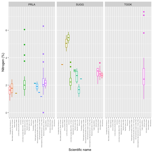
Other Input Options
After downloading the data above, we ran list2env() to make each table
an independent object in the R environment, and then provided the tables
to the two functions as-is. This worked because the names of the objects
were identical to the table names, so the functions were able to figure
out which tables they were. If the object names are not exactly equal to
the table names, you will need to input the table names separately. If
we hadn't used list2env(), this is how we would proceed:
bio.dup <- removeDups(data=apchem$apl_biomass,
variables=apchem$variables_20063,
table="apl_biomass")
chem.dup <- removeDups(data=apchem$apl_plantExternalLabDataPerSample,
variables=apchem$variables_20063,
table="apl_plantExternalLabDataPerSample")
aq.join <- joinTableNEON(table1=bio.dup,
table2=chem.dup,
name1="apl_biomass",
name2="apl_plantExternalLabDataPerSample")
More Complicated Table Joins
In the aquatic plant chemistry example, we were able to join two tables
in a single step. In some cases, the relationship between tables is
more complicated, and joining is more difficult. In these cases,
joinTableNEON() will provide an error message, and usually direct
you to the Quick Start Guide for more information. Let's walk through
how you can use this information, using Mosquitoes sampled from CO2 traps
(DP1.10043.001) from Toolik Lake as an example.
mos <- loadByProduct(dpID="DP1.10043.001",
site="TOOL",
release="RELEASE-2022",
check.size=F)
list2env(mos, .GlobalEnv)
Let's say we're interested in evaluating which mosquito species are found in
which vegetation types. The species identifications are in the
mos_expertTaxonomistIDProcessed table, and the trapping conditions are in
the mos_trapping table. So we'll attempt to join those two tables.
mos.sp <- joinTableNEON(mos_trapping,
mos_expertTaxonomistIDProcessed)
Error in joinTableNEON(mos_trapping, mos_expertTaxonomistIDProcessed) :
Tables mos_trapping and mos_expertTaxonomistIDProcessed can't be joined directly, but can each be joined to a common table(s). Consult quick start guide for details.
The function returns an error, telling us it can't perform a simple join on the two tables, but there is a table they can each join to, which can be used to join them indirectly. As directed, we refer to the Quick Start Guide for DP1.10043.001, on the Data Product Details page.
From the QSG, we learn that mos_sorting is the intermediate table
between mos_trapping and mos_expertTaxonomistIDProcessed.
First, let's join mos_trapping and mos_sorting:
mos.trap <- joinTableNEON(mos_trapping,
mos_sorting)
Now, this next step is a bit odd. We've created a merged table of
mos_trapping and mos_sorting, but we know
mos_expertTaxonomistIDProcessed can only join to mos_sorting. So
we pass the merged table to joinTableNEON(), telling the function to
use the join instructions for mos_sorting and
mos_expertTaxonomistIDProcessed.
mos.tax <- joinTableNEON(mos.trap,
mos_expertTaxonomistIDProcessed,
name1="mos_sorting")
When you join data in this way, check carefully that the resulting table is structured logically and contains the data you expect it to. Looking at the merged table, we now have multiple records for each trapping event, with one record for each species captured in that event, plus a set of records for traps that either caught no mosquitoes or couldn't be deployed, and thus have no species identifications. This is consistent with the table join we performed, so everything appears to be correct.
Let's take a look at species occurrence by habitat, as we set out to do:
gg <- ggplot(mos.tax,
aes(scientificName, individualCount,
group=scientificName,
color=scientificName)) +
geom_boxplot() +
facet_wrap(~nlcdClass) +
theme(axis.text.x=element_blank()) +
ylab("Count") +
xlab("Scientific name")
gg
## Warning: Removed 599 rows containing non-finite values (stat_boxplot).
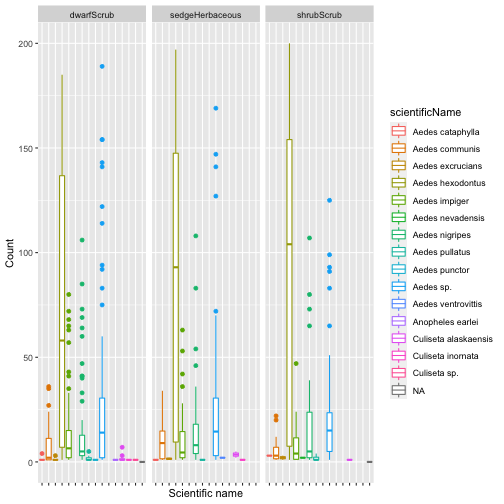
Get Lesson Code
Explore and work with NEON biodiversity data from aquatic ecosystems
Last Updated: Apr 2, 2026
Learning Objectives
After completing this tutorial you will be able to:
- Download NEON macroinvertebrate data.
- Organize those data into long and wide tables.
- Calculate alpha, beta, and gamma diversity following Jost (2007).
Things You’ll Need To Complete This Tutorial
R Programming Language
You will need a current version of R to complete this tutorial. We also recommend the RStudio IDE to work with R.
R Packages to Install
Prior to starting the tutorial ensure that the following packages are installed.
-
tidyverse:
install.packages("tidyverse") -
neonUtilities:
install.packages("neonUtilities") -
vegan:
install.packages("vegan")
More on Packages in R – Adapted from Software Carpentry.
Introduction
Biodiversity is a popular topic within ecology, but quantifying and describing biodiversity precisely can be elusive. In this tutorial, we will describe many of the aspects of biodiversity using NEON's Macroinvertebrate Collection data.
Load Libraries and Prepare Workspace
First, we will load all necessary libraries into our R environment. If you have not already installed these libraries, please see the 'R Packages to Install' section above.
There are also two optional sections in this code chunk: clearing your environment, and loading your NEON API token. Clearing out your environment will erase all of the variables and data that are currently loaded in your R session. This is a good practice for many reasons, but only do this if you are completely sure that you won't be losing any important information! Secondly, your NEON API token will allow you increased download speeds, and helps NEON anonymously track data usage statistics, which helps us optimize our data delivery platforms, and informs our monthly and annual reporting to our funding agency, the National Science Foundation. Please consider signing up for a NEON data user account and using your token as described in this tutorial here.
# clean out workspace
#rm(list = ls()) # OPTIONAL - clear out your environment
#gc() # Uncomment these lines if desired
# load libraries
library(tidyverse)
library(neonUtilities)
library(vegan)
# source .r file with my NEON_TOKEN
# source("my_neon_token.R") # OPTIONAL - load NEON token
# See: https://www.neonscience.org/neon-api-tokens-tutorial
Download NEON Macroinvertebrate Data
Now that the workspace is prepared, we will download NEON macroinvertebrate data using the neonUtilities function loadByProduct().
# Macroinvert dpid
my_dpid <- 'DP1.20120.001'
# list of sites
my_site_list <- c('ARIK', 'POSE', 'MAYF')
# get all tables for these sites from the API -- takes < 1 minute
all_tabs_inv <- neonUtilities::loadByProduct(
dpID = my_dpid,
site = my_site_list,
#token = NEON_TOKEN, #Uncomment to use your token
check.size = F)
Macroinvertebrate Data Munging
Now that we have the data downloaded, we will need to do some 'data munging' to reorganize our data into a more useful format for this analysis. First, let's take a look at some of the tables that were generated by loadByProduct():
# what tables do you get with macroinvertebrate
# data product
names(all_tabs_inv)
## [1] "categoricalCodes_20120" "inv_fieldData" "inv_persample" "inv_taxonomyProcessed" "issueLog_20120"
## [6] "readme_20120" "validation_20120" "variables_20120"
# extract items from list and put in R env.
all_tabs_inv %>% list2env(.GlobalEnv)
## <environment: R_GlobalEnv>
# readme has the same informaiton as what you
# will find on the landing page on the data portal
# The variables file describes each field in
# the returned data tables
View(variables_20120)
# The validation file provides the rules that
# constrain data upon ingest into the NEON database:
View(validation_20120)
# the categoricalCodes file provides controlled
# lists used in the data
View(categoricalCodes_20120)
Next, we will perform several operations in a row to re-organize our data. Each step is described by a code comment.
# It is good to check for duplicate records. This had occurred in the past in
# data published in the inv_fieldData table in 2021. Those duplicates were
# fixed in the 2022 data release.
# Here we use sampleID as primary key and if we find duplicate records, we
# keep the first uid associated with any sampleID that has multiple uids
de_duped_uids <- inv_fieldData %>%
# remove records where no sample was collected
filter(!is.na(sampleID)) %>%
group_by(sampleID) %>%
summarise(n_recs = length(uid),
n_unique_uids = length(unique(uid)),
uid_to_keep = dplyr::first(uid))
# Are there any records that have more than one unique uid?
max_dups <- max(de_duped_uids$n_unique_uids %>% unique())
# filter data using de-duped uids if they exist
if(max_dups > 1){
inv_fieldData <- inv_fieldData %>%
dplyr::filter(uid %in% de_duped_uids$uid_to_keep)
}
# extract year from date, add it as a new column
inv_fieldData <- inv_fieldData %>%
mutate(
year = collectDate %>%
lubridate::as_date() %>%
lubridate::year())
# extract location data into a separate table
table_location <- inv_fieldData %>%
# keep only the columns listed below
select(siteID,
domainID,
namedLocation,
decimalLatitude,
decimalLongitude,
elevation) %>%
# keep rows with unique combinations of values,
# i.e., no duplicate records
distinct()
# create a taxon table, which describes each
# taxonID that appears in the data set
# start with inv_taxonomyProcessed
table_taxon <- inv_taxonomyProcessed %>%
# keep only the coluns listed below
select(acceptedTaxonID, taxonRank, scientificName,
order, family, genus,
identificationQualifier,
identificationReferences) %>%
# remove rows with duplicate information
distinct()
# taxon table information for all taxa in
# our database can be downloaded here:
# takes 1-2 minutes
# full_taxon_table_from_api <- neonUtilities::getTaxonTable("MACROINVERTEBRATE", token = NEON_TOKEN)
# Make the observation table.
# start with inv_taxonomyProcessed
# check for repeated taxa within a sampleID that need to be added together
inv_taxonomyProcessed_summed <- inv_taxonomyProcessed %>%
select(sampleID,
acceptedTaxonID,
individualCount,
estimatedTotalCount) %>%
group_by(sampleID, acceptedTaxonID) %>%
summarize(
across(c(individualCount, estimatedTotalCount), ~sum(.x, na.rm = TRUE)))
# join summed taxon counts back with sample and field data
table_observation <- inv_taxonomyProcessed_summed %>%
# Join relevant sample info back in by sampleID
left_join(inv_taxonomyProcessed %>%
select(sampleID,
domainID,
siteID,
namedLocation,
collectDate,
acceptedTaxonID,
order, family, genus,
scientificName,
taxonRank) %>%
distinct()) %>%
# Join the columns selected above with two
# columns from inv_fieldData (the two columns
# are sampleID and benthicArea)
left_join(inv_fieldData %>%
select(sampleID, eventID, year,
habitatType, samplerType,
benthicArea)) %>%
# some new columns called 'variable_name',
# 'value', and 'unit', and assign values for
# all rows in the table.
# variable_name and unit are both assigned the
# same text strint for all rows.
mutate(inv_dens = estimatedTotalCount / benthicArea,
inv_dens_unit = 'count per square meter')
# check for duplicate records, should return a table with 0 rows
table_observation %>%
group_by(sampleID, acceptedTaxonID) %>%
summarize(n_obs = length(sampleID)) %>%
filter(n_obs > 1)
## # A tibble: 0 x 3
## # Groups: sampleID [0]
## # ... with 3 variables: sampleID <chr>, acceptedTaxonID <chr>, n_obs <int>
# extract sample info
table_sample_info <- table_observation %>%
select(sampleID, domainID, siteID, namedLocation,
collectDate, eventID, year,
habitatType, samplerType, benthicArea,
inv_dens_unit) %>%
distinct()
# remove singletons and doubletons
# create an occurrence summary table
taxa_occurrence_summary <- table_observation %>%
select(sampleID, acceptedTaxonID) %>%
distinct() %>%
group_by(acceptedTaxonID) %>%
summarize(occurrences = n())
# filter out taxa that are only observed 1 or 2 times
taxa_list_cleaned <- taxa_occurrence_summary %>%
filter(occurrences > 2)
# filter observation table based on taxon list above
table_observation_cleaned <- table_observation %>%
filter(acceptedTaxonID %in%
taxa_list_cleaned$acceptedTaxonID,
!sampleID %in% c("MAYF.20190729.CORE.1",
"MAYF.20200713.CORE.1",
"MAYF.20210721.CORE.1",
"POSE.20160718.HESS.1"))
#this is an outlier sampleID
# some summary data
sampling_effort_summary <- table_sample_info %>%
# group by siteID, year
group_by(siteID, year, samplerType) %>%
# count samples and habitat types within each event
summarise(
event_count = eventID %>% unique() %>% length(),
sample_count = sampleID %>% unique() %>% length(),
habitat_count = habitatType %>%
unique() %>% length())
# check out the summary table
sampling_effort_summary %>% as.data.frame() %>%
head() %>% print()
## siteID year samplerType event_count sample_count habitat_count
## 1 ARIK 2014 core 2 6 1
## 2 ARIK 2014 modifiedKicknet 2 10 1
## 3 ARIK 2015 core 3 11 2
## 4 ARIK 2015 modifiedKicknet 3 13 2
## 5 ARIK 2016 core 3 9 1
## 6 ARIK 2016 modifiedKicknet 3 15 1
Working with 'Long' data
'Reshaping' your data to use as an input to a particular fuction may require you to consider: do I want 'long' or 'wide' data? Here's a link to a great article from 'the analysis factor' that describes the differences.
For this first step, we will use data in a 'long' table:
# no. taxa by rank by site
table_observation_cleaned %>%
group_by(domainID, siteID, taxonRank) %>%
summarize(
n_taxa = acceptedTaxonID %>%
unique() %>% length()) %>%
ggplot(aes(n_taxa, taxonRank)) +
facet_wrap(~ domainID + siteID) +
geom_col()
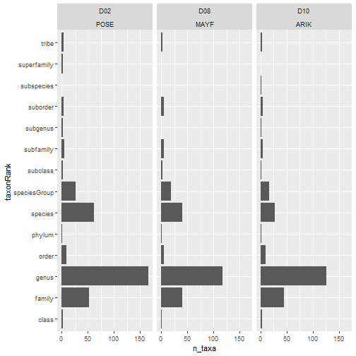
# library(scales)
# sum densities by order for each sampleID
table_observation_by_order <-
table_observation_cleaned %>%
filter(!is.na(order)) %>%
group_by(domainID, siteID, year,
eventID, sampleID, habitatType, order) %>%
summarize(order_dens = sum(inv_dens, na.rm = TRUE))
# rank occurrence by order
table_observation_by_order %>% head()
## # A tibble: 6 x 8
## # Groups: domainID, siteID, year, eventID, sampleID, habitatType [1]
## domainID siteID year eventID sampleID habitatType order order_dens
## <chr> <chr> <dbl> <chr> <chr> <chr> <chr> <dbl>
## 1 D02 POSE 2014 POSE.20140722 POSE.20140722.SURBER.1 riffle Branchiobdellida 516.
## 2 D02 POSE 2014 POSE.20140722 POSE.20140722.SURBER.1 riffle Coleoptera 516.
## 3 D02 POSE 2014 POSE.20140722 POSE.20140722.SURBER.1 riffle Decapoda 86.0
## 4 D02 POSE 2014 POSE.20140722 POSE.20140722.SURBER.1 riffle Diptera 5419.
## 5 D02 POSE 2014 POSE.20140722 POSE.20140722.SURBER.1 riffle Ephemeroptera 5301.
## 6 D02 POSE 2014 POSE.20140722 POSE.20140722.SURBER.1 riffle Megaloptera 387.
# stacked rank occurrence plot
table_observation_by_order %>%
group_by(order, siteID) %>%
summarize(
occurrence = (order_dens > 0) %>% sum()) %>%
ggplot(aes(
x = reorder(order, -occurrence),
y = occurrence,
color = siteID,
fill = siteID)) +
geom_col() +
theme(axis.text.x =
element_text(angle = 45, hjust = 1))
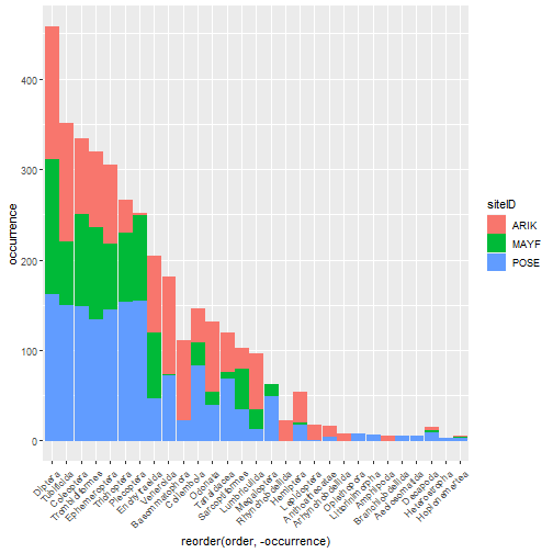
# faceted densities plot
table_observation_by_order %>%
ggplot(aes(
x = reorder(order, -order_dens),
y = log10(order_dens),
color = siteID,
fill = siteID)) +
geom_boxplot(alpha = .5) +
facet_grid(siteID ~ .) +
theme(axis.text.x =
element_text(angle = 45, hjust = 1))
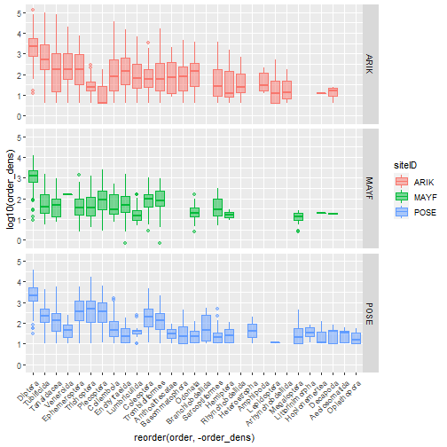
Making Data 'wide'
For the next process, we will need to make our data table in the 'wide' format.
# select only site by species density info and remove duplicate records
table_sample_by_taxon_density_long <- table_observation_cleaned %>%
select(sampleID, acceptedTaxonID, inv_dens) %>%
distinct() %>%
filter(!is.na(inv_dens))
# table_sample_by_taxon_density_long %>% nrow()
# table_sample_by_taxon_density_long %>% distinct() %>% nrow()
# pivot to wide format, sum multiple counts per sampleID
table_sample_by_taxon_density_wide <- table_sample_by_taxon_density_long %>%
tidyr::pivot_wider(id_cols = sampleID,
names_from = acceptedTaxonID,
values_from = inv_dens,
values_fill = list(inv_dens = 0),
values_fn = list(inv_dens = sum)) %>%
column_to_rownames(var = "sampleID")
# check col and row sums -- mins should all be > 0
colSums(table_sample_by_taxon_density_wide) %>% min()
## [1] 12
rowSums(table_sample_by_taxon_density_wide) %>% min()
## [1] 25.55004
Multiscale Biodiversity
Reference: Jost, L. 2007. Partitioning diversity into independent alpha and beta components. Ecology 88:2427–2439. https://doi.org/10.1890/06-1736.1.
These metrics are based on Robert Whittaker's multiplicative diversity where
- gamma is regional biodiversity
- alpha is local biodiversity (e.g., the mean diversity at a patch)
- and beta diversity is a measure of among-patch variability in community composition.
Beta could be interpreted as the number of "distinct" communities present within the region.
The relationship among alpha, beta, and gamma diversity is: beta = gamma / alpha
The influence of relative abundances over the calculation of alpha, beta, and gamma diversity metrics is determined by the coefficient q. The coefficient "q" determines the "order" of the diversity metric, where q = 0 provides diversity measures based on richness, and higher orders of q give more weight to taxa that have higher abundances in the data. Order q = 1 is related to Shannon diveristy metrics, and order q = 2 is related to Simpson diversity metrics.
Alpha diversity is average local richness.
Order q = 0 alpha diversity calculated for our dataset returns a mean local richness (i.e., species counts) of ~30 taxa per sample across the entire data set.
# Here we use vegan::renyi to calculate Hill numbers
# If hill = FALSE, the function returns an entropy
# If hill = TRUE, the function returns the exponentiated
# entropy. In other words:
# exp(renyi entropy) = Hill number = "species equivalent"
# Note that for this function, the "scales" argument
# determines the order of q used in the calculation
table_sample_by_taxon_density_wide %>%
vegan::renyi(scales = 0, hill = TRUE) %>%
mean()
## [1] 30.06114
Comparing alpha diversity calculated using different orders:
Order q = 1 alpha diversity returns mean number of "species equivalents" per sample in the data set. This approach incorporates evenness because when abundances are more even across taxa, taxa are weighted more equally toward counting as a "species equivalent". For example, if you have a sample with 100 individuals, spread across 10 species, and each species is represented by 10 individuals, the number of order q = 1 species equivalents will equal the richness (10).
Alternatively, if 90 of the 100 individuals in the sample are one species, and the other 10 individuals are spread across the other 9 species, there will only be 1.72 order q = 1 species equivalents, whereas, there are still 10 species in the sample.
# even distribution, orders q = 0 and q = 1 for 10 taxa
vegan::renyi(
c(spp.a = 10, spp.b = 10, spp.c = 10,
spp.d = 10, spp.e = 10, spp.f = 10,
spp.g = 10, spp.h = 10, spp.i = 10,
spp.j = 10),
hill = TRUE,
scales = c(0, 1))
## 0 1
## 10 10
## attr(,"class")
## [1] "renyi" "numeric"
# uneven distribution, orders q = 0 and q = 1 for 10 taxa
vegan::renyi(
c(spp.a = 90, spp.b = 2, spp.c = 1,
spp.d = 1, spp.e = 1, spp.f = 1,
spp.g = 1, spp.h = 1, spp.i = 1,
spp.j = 1),
hill = TRUE,
scales = c(0, 1))
## 0 1
## 10.000000 1.718546
## attr(,"class")
## [1] "renyi" "numeric"
Comparing orders of q for NEON data
Let's compare the different orders q = 0, 1, and 2 measures of alpha diversity across the samples collected from ARIK, POSE, and MAYF.
# Nest data by siteID
data_nested_by_siteID <- table_sample_by_taxon_density_wide %>%
tibble::rownames_to_column("sampleID") %>%
left_join(table_sample_info %>%
select(sampleID, siteID)) %>%
tibble::column_to_rownames("sampleID") %>%
nest(data = -siteID)
data_nested_by_siteID$data[[1]] %>%
vegan::renyi(scales = 0, hill = TRUE) %>%
mean()
## [1] 24.69388
# apply the calculation by site for alpha diversity
# for each order of q
data_nested_by_siteID %>% mutate(
alpha_q0 = purrr::map_dbl(
.x = data,
.f = ~ vegan::renyi(x = .,
hill = TRUE,
scales = 0) %>% mean()),
alpha_q1 = purrr::map_dbl(
.x = data,
.f = ~ vegan::renyi(x = .,
hill = TRUE,
scales = 1) %>% mean()),
alpha_q2 = purrr::map_dbl(
.x = data,
.f = ~ vegan::renyi(x = .,
hill = TRUE,
scales = 2) %>% mean())
)
## # A tibble: 3 x 5
## siteID data alpha_q0 alpha_q1 alpha_q2
## <chr> <list> <dbl> <dbl> <dbl>
## 1 ARIK <tibble [147 x 458]> 24.7 10.2 6.52
## 2 MAYF <tibble [149 x 458]> 22.2 12.0 8.19
## 3 POSE <tibble [162 x 458]> 42.1 20.7 13.0
# Note that POSE has the highest mean alpha diversity
# To calculate gamma diversity at the site scale,
# calculate the column means and then calculate
# the renyi entropy and Hill number
# Here we are only calcuating order
# q = 0 gamma diversity
data_nested_by_siteID %>% mutate(
gamma_q0 = purrr::map_dbl(
.x = data,
.f = ~ vegan::renyi(x = colMeans(.),
hill = TRUE,
scales = 0)))
## # A tibble: 3 x 3
## siteID data gamma_q0
## <chr> <list> <dbl>
## 1 ARIK <tibble [147 x 458]> 243
## 2 MAYF <tibble [149 x 458]> 239
## 3 POSE <tibble [162 x 458]> 337
# Note that POSE has the highest gamma diversity
# Now calculate alpha, beta, and gamma using orders 0 and 1
# for each siteID
diversity_partitioning_results <-
data_nested_by_siteID %>%
mutate(
n_samples = purrr::map_int(data, ~ nrow(.)),
alpha_q0 = purrr::map_dbl(
.x = data,
.f = ~ vegan::renyi(x = .,
hill = TRUE,
scales = 0) %>% mean()),
alpha_q1 = purrr::map_dbl(
.x = data,
.f = ~ vegan::renyi(x = .,
hill = TRUE,
scales = 1) %>% mean()),
gamma_q0 = purrr::map_dbl(
.x = data,
.f = ~ vegan::renyi(x = colMeans(.),
hill = TRUE,
scales = 0)),
gamma_q1 = purrr::map_dbl(
.x = data,
.f = ~ vegan::renyi(x = colMeans(.),
hill = TRUE,
scales = 1)),
beta_q0 = gamma_q0 / alpha_q0,
beta_q1 = gamma_q1 / alpha_q1)
diversity_partitioning_results %>%
select(-data) %>% as.data.frame() %>% print()
## siteID n_samples alpha_q0 alpha_q1 gamma_q0 gamma_q1 beta_q0 beta_q1
## 1 ARIK 147 24.69388 10.19950 243 35.70716 9.840496 3.500873
## 2 MAYF 149 22.24832 12.02405 239 65.77590 10.742383 5.470360
## 3 POSE 162 42.11728 20.70184 337 100.16506 8.001466 4.838462
Using NMDS to ordinate samples
Finally, we will use Nonmetric Multidimensional Scaling (NMDS) to ordinate samples as shown below:
# create ordination using NMDS
my_nmds_result <- table_sample_by_taxon_density_wide %>% vegan::metaMDS()
## Square root transformation
## Wisconsin double standardization
## Run 0 stress 0.2280867
## Run 1 stress 0.2297516
## Run 2 stress 0.2322618
## Run 3 stress 0.2492232
## Run 4 stress 0.2335912
## Run 5 stress 0.235082
## Run 6 stress 0.2396413
## Run 7 stress 0.2303469
## Run 8 stress 0.2363123
## Run 9 stress 0.2523796
## Run 10 stress 0.2288613
## Run 11 stress 0.2302371
## Run 12 stress 0.2302613
## Run 13 stress 0.2409554
## Run 14 stress 0.2308922
## Run 15 stress 0.2528171
## Run 16 stress 0.2534587
## Run 17 stress 0.2320313
## Run 18 stress 0.239435
## Run 19 stress 0.2293618
## Run 20 stress 0.2307903
## *** No convergence -- monoMDS stopping criteria:
## 1: no. of iterations >= maxit
## 18: stress ratio > sratmax
## 1: scale factor of the gradient < sfgrmin
# plot stress
my_nmds_result$stress
## [1] 0.2280867
p1 <- vegan::ordiplot(my_nmds_result)
vegan::ordilabel(p1, "species")
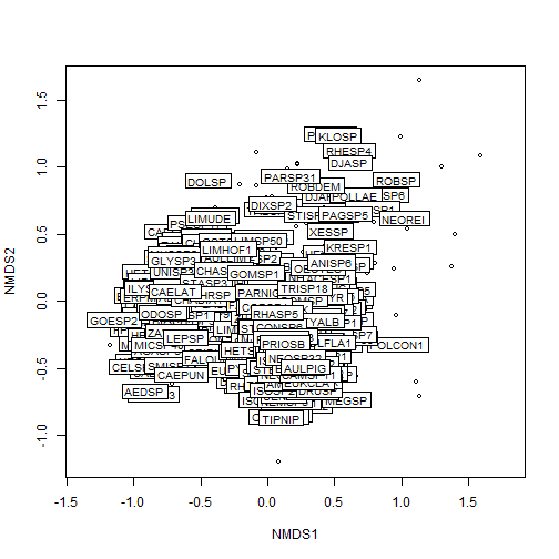
# merge NMDS scores with sampleID information for plotting
nmds_scores <- my_nmds_result %>%
vegan::scores() %>%
.[["sites"]] %>%
as.data.frame() %>%
tibble::rownames_to_column("sampleID") %>%
left_join(table_sample_info)
# # How I determined the outlier(s)
nmds_scores %>% arrange(desc(NMDS1)) %>% head()
## sampleID NMDS1 NMDS2 domainID siteID namedLocation collectDate eventID year habitatType
## 1 MAYF.20190311.CORE.2 1.590745 1.0833382 D08 MAYF MAYF.AOS.reach 2019-03-11 15:00:00 MAYF.20190311 2019 run
## 2 MAYF.20201117.CORE.2 1.395784 0.4986856 D08 MAYF MAYF.AOS.reach 2020-11-17 16:33:00 MAYF.20201117 2020 run
## 3 MAYF.20180726.CORE.2 1.372494 0.2603682 D08 MAYF MAYF.AOS.reach 2018-07-26 14:17:00 MAYF.20180726 2018 run
## 4 MAYF.20190311.CORE.1 1.299395 1.0075703 D08 MAYF MAYF.AOS.reach 2019-03-11 15:00:00 MAYF.20190311 2019 run
## 5 MAYF.20170314.CORE.1 1.132679 1.6469463 D08 MAYF MAYF.AOS.reach 2017-03-14 14:11:00 MAYF.20170314 2017 run
## 6 MAYF.20180326.CORE.3 1.130687 -0.7139679 D08 MAYF MAYF.AOS.reach 2018-03-26 14:50:00 MAYF.20180326 2018 run
## samplerType benthicArea inv_dens_unit
## 1 core 0.006 count per square meter
## 2 core 0.006 count per square meter
## 3 core 0.006 count per square meter
## 4 core 0.006 count per square meter
## 5 core 0.006 count per square meter
## 6 core 0.006 count per square meter
nmds_scores %>% arrange(desc(NMDS1)) %>% tail()
## sampleID NMDS1 NMDS2 domainID siteID namedLocation collectDate eventID year habitatType
## 453 ARIK.20160919.KICKNET.5 -0.8577931 -0.245144245 D10 ARIK ARIK.AOS.reach 2016-09-19 22:06:00 ARIK.20160919 2016 run
## 454 ARIK.20160919.KICKNET.1 -0.8694139 0.291753483 D10 ARIK ARIK.AOS.reach 2016-09-19 22:06:00 ARIK.20160919 2016 run
## 455 ARIK.20150714.CORE.3 -0.8843672 0.013601377 D10 ARIK ARIK.AOS.reach 2015-07-14 14:55:00 ARIK.20150714 2015 pool
## 456 ARIK.20150714.CORE.2 -1.0465497 0.004066437 D10 ARIK ARIK.AOS.reach 2015-07-14 14:55:00 ARIK.20150714 2015 pool
## 457 ARIK.20160919.KICKNET.4 -1.0937181 -0.148046639 D10 ARIK ARIK.AOS.reach 2016-09-19 22:06:00 ARIK.20160919 2016 run
## 458 ARIK.20160331.CORE.3 -1.1791981 -0.327145374 D10 ARIK ARIK.AOS.reach 2016-03-31 15:41:00 ARIK.20160331 2016 pool
## samplerType benthicArea inv_dens_unit
## 453 modifiedKicknet 0.250 count per square meter
## 454 modifiedKicknet 0.250 count per square meter
## 455 core 0.006 count per square meter
## 456 core 0.006 count per square meter
## 457 modifiedKicknet 0.250 count per square meter
## 458 core 0.006 count per square meter
# Plot samples in community composition space by year
nmds_scores %>%
ggplot(aes(NMDS1, NMDS2, color = siteID,
shape = samplerType)) +
geom_point() +
facet_wrap(~ as.factor(year))
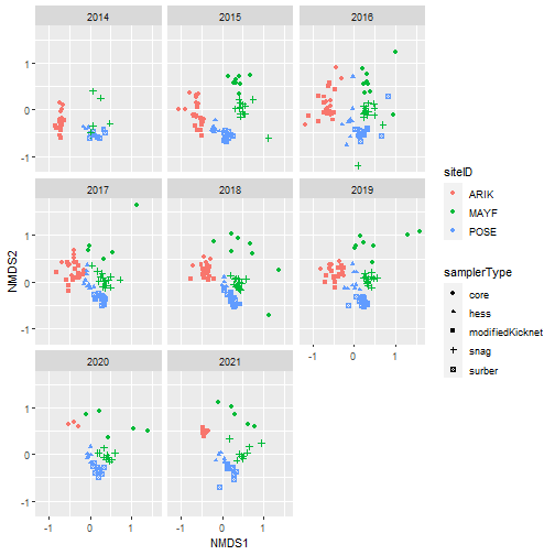
# Plot samples in community composition space
# facet by siteID and habitat type
# color by year
nmds_scores %>%
ggplot(aes(NMDS1, NMDS2, color = as.factor(year),
shape = samplerType)) +
geom_point() +
facet_grid(habitatType ~ siteID, scales = "free")
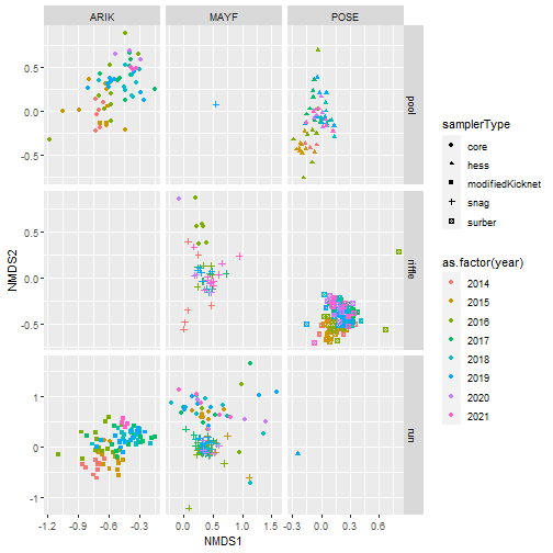
Get Lesson Code
Create a Canopy Height Model from Lidar-derived rasters in R
Last Updated: Apr 2, 2026
A common analysis using lidar data are to derive top of the canopy height values from the lidar data. These values are often used to track changes in forest structure over time, to calculate biomass, and even leaf area index (LAI). Let's dive into the basics of working with raster formatted lidar data in R!
Learning Objectives
After completing this tutorial, you will be able to:
- Work with digital terrain model (DTM) & digital surface model (DSM) raster files.
- Create a canopy height model (CHM) raster from DTM & DSM rasters.
Things You’ll Need To Complete This Tutorial
You will need the most current version of R and, preferably, RStudio loaded
on your computer to complete this tutorial.
Install R Packages
-
terra:
install.packages("terra") -
neonUtilities:
install.packages("neonUtilities")
More on Packages in R - Adapted from Software Carpentry.
Download Data
Lidar elevation raster data are downloaded using the R neonUtilities::byTileAOP function in the script.
These remote sensing data files provide information on the vegetation at the National Ecological Observatory Network's San Joaquin Experimental Range and Soaproot Saddle field sites. The entire datasets can be accessed from the NEON Data Portal.
This tutorial is designed for you to set your working directory to the directory created by unzipping this file.
Set Working Directory: This lesson will walk you through setting the working directory before downloading the datasets from neonUtilities.
An overview of setting the working directory in R can be found here.
R Script & Challenge Code: NEON data lessons often contain challenges to reinforce skills. If available, the code for challenge solutions is found in the downloadable R script of the entire lesson, available in the footer of each lesson page.
Recommended Reading
What is a CHM, DSM and DTM? About Gridded, Raster LiDAR DataCreate a lidar-derived Canopy Height Model (CHM)
The National Ecological Observatory Network (NEON) will provide lidar-derived data products as one of its many free ecological data products. These products will come in the GeoTIFF format, which is a .tif raster format that is spatially located on the earth.
In this tutorial, we create a Canopy Height Model. The Canopy Height Model (CHM), represents the heights of the trees on the ground. We can derive the CHM by subtracting the ground elevation from the elevation of the top of the surface (or the tops of the trees).
We will use the terra R package to work with the the lidar-derived Digital
Surface Model (DSM) and the Digital Terrain Model (DTM).
# Load needed packages
library(terra)
library(neonUtilities)
Set the working directory so you know where to download data.
wd="~/data/" #This will depend on your local environment
setwd(wd)
We can use the neonUtilities function byTileAOP to download a single DTM and DSM tile at SJER. Both the DTM and DSM are delivered under the Elevation - LiDAR (DP3.30024.001) data product.
You can run help(byTileAOP) to see more details on what the various inputs are. For this exercise, we'll specify the UTM Easting and Northing to be (257500, 4112500), which will download the tile with the lower left corner (257000,4112000). By default, the function will check the size total size of the download and ask you whether you wish to proceed (y/n). You can set check.size=FALSE if you want to download without a prompt. This example will not be very large (~8MB), since it is only downloading two single-band rasters (plus some associated metadata).
byTileAOP(dpID='DP3.30024.001',
site='SJER',
year='2021',
easting=257500,
northing=4112500,
check.size=TRUE, # set to FALSE if you don't want to enter y/n
savepath = wd)
This file will be downloaded into a nested subdirectory under the ~/data folder, inside a folder named DP3.30024.001 (the Data Product ID). The files should show up in these locations: ~/data/DP3.30024.001/neon-aop-products/2021/FullSite/D17/2021_SJER_5/L3/DiscreteLidar/DSMGtif/NEON_D17_SJER_DP3_257000_4112000_DSM.tif and ~/data/DP3.30024.001/neon-aop-products/2021/FullSite/D17/2021_SJER_5/L3/DiscreteLidar/DTMGtif/NEON_D17_SJER_DP3_257000_4112000_DTM.tif.
Now we can read in the files. You can move the files to a different location (eg. shorten the path), but make sure to change the path that points to the file accordingly.
# Define the DSM and DTM file names, including the full path
dsm_file <- paste0(wd,"DP3.30024.001/neon-aop-products/2021/FullSite/D17/2021_SJER_5/L3/DiscreteLidar/DSMGtif/NEON_D17_SJER_DP3_257000_4112000_DSM.tif")
dtm_file <- paste0(wd,"DP3.30024.001/neon-aop-products/2021/FullSite/D17/2021_SJER_5/L3/DiscreteLidar/DTMGtif/NEON_D17_SJER_DP3_257000_4112000_DTM.tif")
First, we will read in the Digital Surface Model (DSM). The DSM represents the elevation of the top of the objects on the ground (trees, buildings, etc).
# assign raster to object
dsm <- rast(dsm_file)
# view info about the raster.
dsm
## class : SpatRaster
## dimensions : 1000, 1000, 1 (nrow, ncol, nlyr)
## resolution : 1, 1 (x, y)
## extent : 257000, 258000, 4112000, 4113000 (xmin, xmax, ymin, ymax)
## coord. ref. : WGS 84 / UTM zone 11N (EPSG:32611)
## source : NEON_D17_SJER_DP3_257000_4112000_DSM.tif
## name : NEON_D17_SJER_DP3_257000_4112000_DSM
# plot the DSM
plot(dsm, main="Lidar Digital Surface Model \n SJER, California")
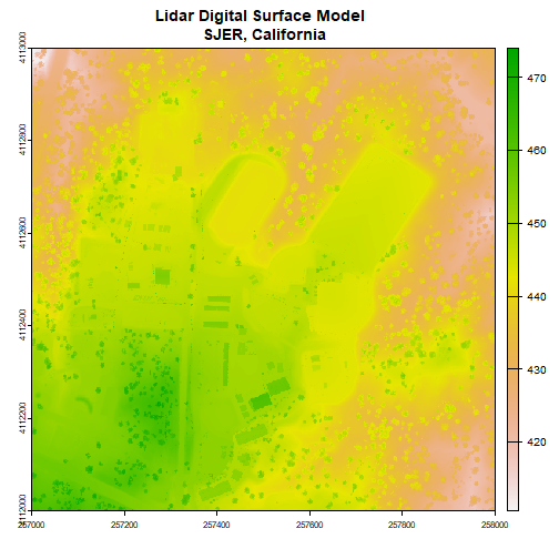
Note the resolution, extent, and coordinate reference system (CRS) of the raster. To do later steps, our DTM will need to be the same.
Next, we will import the Digital Terrain Model (DTM) for the same area. The DTM represents the ground (terrain) elevation.
# import the digital terrain model
dtm <- rast(dtm_file)
plot(dtm, main="Lidar Digital Terrain Model \n SJER, California")
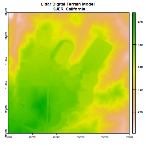
With both of these rasters now loaded, we can create the Canopy Height Model (CHM). The CHM represents the difference between the DSM and the DTM or the height of all objects on the surface of the earth.
To do this we perform some basic raster math to calculate the CHM. You can perform the same raster math in a GIS program like QGIS.
When you do the math, make sure to subtract the DTM from the DSM or you'll get trees with negative heights!
# use raster math to create CHM
chm <- dsm - dtm
# view CHM attributes
chm
## class : SpatRaster
## dimensions : 1000, 1000, 1 (nrow, ncol, nlyr)
## resolution : 1, 1 (x, y)
## extent : 257000, 258000, 4112000, 4113000 (xmin, xmax, ymin, ymax)
## coord. ref. : WGS 84 / UTM zone 11N (EPSG:32611)
## source(s) : memory
## varname : NEON_D17_SJER_DP3_257000_4112000_DSM
## name : NEON_D17_SJER_DP3_257000_4112000_DSM
## min value : 0.00
## max value : 24.13
plot(chm, main="Lidar CHM - SJER, California")
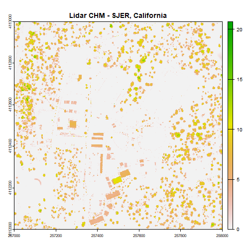
We've now created a CHM from our DSM and DTM. What do you notice about the canopy cover at this location in the San Joaquin Experimental Range?
Challenge: Basic Raster Math
Convert the CHM from meters to feet and plot it.
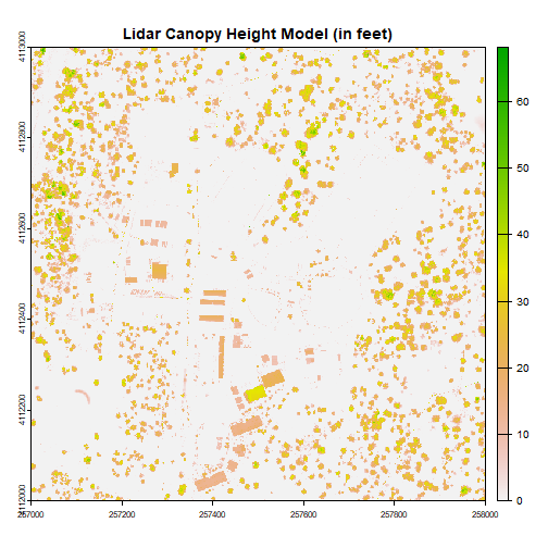
We can write out the CHM as a GeoTiff using the writeRaster() function.
# write out the CHM in tiff format.
writeRaster(chm,paste0(wd,"CHM_SJER.tif"),"GTiff")
We've now successfully created a canopy height model using basic raster math -- in
R! We can bring the CHM_SJER.tif file into QGIS (or any GIS program) and look
at it.
Consider checking out the tutorial Compare tree height measured from the ground to a Lidar-based Canopy Height Model to compare a LiDAR-derived CHM with ground-based observations!
Get Lesson Code
Compare tree height measured from the ground to a Lidar-based Canopy Height Model
Last Updated: Apr 2, 2026
An extremely common task for remote sensing researchers is to connect remote sensing data with data on the ground. This might be a research question in itself - what reflectance wavelengths are most closely correlated with a particular ground feature? - or a ground-truthing for extrapolation and prediction, or development or testing of a model.
This tutorial explores the relationship between a Lidar-derived canopy height model and tree heights measured from the ground, because these two datasets provide a straightforward introduction to thinking about how to relate different sources of data. They are a good exemplar for the two major components of connecting airborne and ground data:
- The mechanics: Finding the remotely sensed pixels that correspond to a given ground measurement
- The science: Considering biases in each data source, and the ways the measurements might differ even if neither is incorrect
We will explore these issues between these two datasets, and you can use what you learn here as a roadmap for making similar comparisons between different datasets.
The two NEON data products that estimate tree height:
- DP3.30015.001, Ecosystem structure, aka Canopy Height Model (CHM)
- DP1.10098.001, Vegetation structure
The CHM data are derived from the Lidar point cloud data collected by the remote sensing platform. The vegetation structure data are collected by by field staff on the ground.
We will be using data from the Wind River Experimental Forest (WREF) NEON field site located in Washington state. The predominant vegetation there is tall evergreen conifers.
Things You’ll Need To Complete This Tutorial
You will need the a recent version of R (4+) or Python (3.9+) loaded on your computer to complete this tutorial.
1. Setup
Start by installing and loading packages (if necessary) and setting options. Installation can be run once, then periodically to get package updates.
R
One of the packages we’ll be using, geoNEON, is only
available via GitHub, so it’s installed using the devtools
package. The other packages can be installed directly from CRAN.
install.packages("neonUtilities")
install.packages("neonOS")
install.packages("terra")
install.packages("devtools")
devtools::install_github("NEONScience/NEON-geolocation/geoNEON")Now load packages. This needs to be done every time you run code. We’ll also set a working directory for data downloads (adapt the working directory path for your system).
library(terra)
library(neonUtilities)
library(neonOS)
library(geoNEON)
options(stringsAsFactors=F)
wd <- "~/data"
Python
There are a variety of spatial packages available in Python; we’ll
use rasterio and rioxarray. We’ll also use
several modules that are installed automatically with standard Python
installations.
pip install neonutilities
pip install geopandas
pip install rasterio
pip install rioxarray
pip install rasterstatsNow load packages.
import neonutilities as nu
import pandas as pd
import numpy as np
import rasterstats as rs
import geopandas as gpd
import rioxarray as rxr
import matplotlib.pyplot as plt
import matplotlib.collections
import rasterio
from rasterio import sample
from rasterio.enums import Resampling
import requests
import time
import os2. Vegetation structure data
In this section we’ll download the vegetation structure data, find the locations of the mapped trees, and join to the species and size data.
R
Download the vegetation structure data using the
loadByProduct() function in the neonUtilities
package. Inputs to the function are:
dpID: data product ID; woody vegetation structure = DP1.10098.001site: (vector of) 4-letter site codes; Wind River = WREFpackage: basic or expanded; we’ll download basic hererelease: which data release to download; we’ll use RELEASE-2023check.size: should this function prompt the user with an estimated download size? Set toFALSEhere for ease of processing as a script, but good to leave as defaultTRUEwhen downloading a dataset for the first time.
Refer to the
cheat
sheet for the neonUtilities package for more details
and the complete index of possible function inputs.
veglist <- loadByProduct(dpID="DP1.10098.001",
site="WREF",
package="basic",
release="RELEASE-2024",
check.size = FALSE)Python
Download the vegetation structure data using the
load_by_product() function in the
neonutilities package. Inputs to the function are:
dpid: data product ID; woody vegetation structure = DP1.10098.001site: (vector of) 4-letter site codes; Wind River = WREFpackage: basic or expanded; we’ll download basic hererelease: which data release to download; we’ll use RELEASE-2023check_size: should this function prompt the user with an estimated download size? Set toFalsehere for ease of processing as a script, but good to leave as defaultTruewhen downloading a dataset for the first time.
Refer to the
cheat
sheet for the neonUtilities package for more details
and the complete index of possible function inputs. The cheat sheet is
focused on the R package, but nearly all the inputs are the same.
veglist = nu.load_by_product(dpid="DP1.10098.001",
site="WREF",
package="basic",
release="RELEASE-2024",
check_size = False)Get tree locations
R
Use the getLocTOS() function in the geoNEON
package to get precise locations for the tagged plants. Refer to the
package documentation for more details.
vegmap <- getLocTOS(veglist$vst_mappingandtagging,
"vst_mappingandtagging")## Please note locations will be calculated only for mapped woody individuals. To find subplot locations for unmapped individuals, use this function with the vst_apparentindividual, vst_non-woody, and/or vst_shrubgroup tables.Python
NEON doesn’t currently offer a Python equivalent to the
geoNEON R package, so we’ll calculate the tree locations
step-by-step. The trees are mapped as distance and azimuth from a
reference location. The reference location data are accessible on the
NEON API. The steps in this calculation are described in the
Data
Product User Guide.
First, get the names of the reference locations, and query the NEON API to retrieve their location data:
vegmapall = veglist["vst_mappingandtagging"]
vegmap = vegmapall.loc[vegmapall["pointID"] != ""]
vegmap = vegmap.reindex()
vegmap["points"] = vegmap["namedLocation"] + "." + vegmap["pointID"]
veg_points = list(set(list(vegmap["points"])))
easting = []
northing = []
coord_uncertainty = []
elev_uncertainty = []
drop_points = []
for i in veg_points:
time.sleep(1)
vres = requests.get("https://data.neonscience.org/api/v0/locations/"+i)
vres_json = vres.json()
if vres_json["data"] is not None:
easting.append(vres_json["data"]["locationUtmEasting"])
northing.append(vres_json["data"]["locationUtmNorthing"])
props = pd.DataFrame.from_dict(vres_json["data"]["locationProperties"])
cu = props.loc[props["locationPropertyName"] == "Value for Coordinate uncertainty"]["locationPropertyValue"]
coord_uncertainty.append(cu[cu.index[0]])
eu = props.loc[props["locationPropertyName"] == "Value for Elevation uncertainty"]["locationPropertyValue"]
elev_uncertainty.append(eu[eu.index[0]])
else:
drop_points.append(i)
veg_points_clean = [v for v in veg_points if v not in drop_points]
ptdct = dict(points=veg_points_clean,
easting=easting,
northing=northing,
coordinateUncertainty=coord_uncertainty,
elevationUncertainty=elev_uncertainty)
ptfrm = pd.DataFrame.from_dict(ptdct)
ptfrm.set_index("points", inplace=True)
vegmap = vegmap.join(ptfrm,
on="points",
how="inner")Next, use the distance and azimuth data to calculate the precise locations of individuals, relative to the reference locations.
vegmap["adjEasting"] = (vegmap["easting"]
+ vegmap["stemDistance"]
* np.sin(vegmap["stemAzimuth"]
* np.pi / 180))
vegmap["adjNorthing"] = (vegmap["northing"]
+ vegmap["stemDistance"]
* np.cos(vegmap["stemAzimuth"]
* np.pi / 180))
Add to the uncertainty estimate to account for error in measurement from the reference location, as described in the User Guide.
vegmap["adjCoordinateUncertainty"] = vegmap["coordinateUncertainty"] + 0.6
vegmap["adjElevationUncertainty"] = vegmap["elevationUncertainty"] + 1Combine location with tree traits
Now we have the mapped locations of individuals in the
vst_mappingandtagging table, and the annual measurements of
tree dimensions such as height and diameter in the
vst_apparentindividual table. To bring these measurements
together, join the two tables, using the joinTableNEON()
function from the neonOS package. Refer to the
Quick
Start Guide for Vegetation structure for more information about the
data tables and the joining instructions joinTableNEON() is
using.
R
veg <- joinTableNEON(veglist$vst_apparentindividual,
vegmap,
name1="vst_apparentindividual",
name2="vst_mappingandtagging")Python
Like the geoNEON package, there is not currently a
Python equivalent to the neonOS package. Refer to the
Quick
Start Guide for Vegetation structure to find the data field to use
to join the two tables.
veglist["vst_apparentindividual"].set_index("individualID", inplace=True)
veg = vegmap.join(veglist["vst_apparentindividual"],
on="individualID",
how="inner",
lsuffix="_MAT",
rsuffix="_AI")Make a stem map
Let’s see what the data look like! Make a stem map, where each tree is mapped by a circle matching its size. This won’t look informative at the scale of the entire site, so we’ll subset to a single plot, WREF_075.
In addition to looking at only one plot, we’ll also target a single
year. We want to match height measurements from the ground to remote
sensing flights, so we need to pick a year when WREF was flown. We’ll
use 2017. Use the eventID field from
vst_apparentindividual to find the 2017 measurements. We
use the eventID rather than the date because
sampling bouts for vegetation structure are carried out in the winter,
to avoid the growing season, and can sometimes extend into the following
calendar year.
Note that in both languages the input to the function that draws a
circle is a radius, but stemDiameter is just that, a
diameter, so we will need to divide by two. And
stemDiameter is in centimeters, but the mapping scale is in
meters, so we also need to divide by 100 to get the scale right.
R
veg2017 <- veg[which(veg$eventID.y=="vst_WREF_2017"),]
symbols(veg2017$adjEasting[which(veg2017$plotID=="WREF_075")],
veg2017$adjNorthing[which(veg2017$plotID=="WREF_075")],
circles=veg2017$stemDiameter[which(veg2017$plotID=="WREF_075")]/100/2,
inches=F, xlab="Easting", ylab="Northing")

And now overlay the estimated uncertainty in the location of each stem, in blue:
symbols(veg2017$adjEasting[which(veg2017$plotID=="WREF_075")],
veg2017$adjNorthing[which(veg2017$plotID=="WREF_075")],
circles=veg2017$stemDiameter[which(veg2017$plotID=="WREF_075")]/100/2,
inches=F, xlab="Easting", ylab="Northing")
symbols(veg2017$adjEasting[which(veg2017$plotID=="WREF_075")],
veg2017$adjNorthing[which(veg2017$plotID=="WREF_075")],
circles=veg2017$adjCoordinateUncertainty[which(veg2017$plotID=="WREF_075")],
inches=F, add=T, fg="lightblue")
Python
veg2017 = veg.loc[veg["eventID_AI"]=="vst_WREF_2017"]
veg75 = veg2017.loc[veg2017["plotID_AI"]=="WREF_075"]
fig, ax = plt.subplots()
xy = np.array(tuple(zip(veg75.adjEasting, veg75.adjNorthing)))
srad = veg75.stemDiameter/100/2
patches = [plt.Circle(center, size) for center, size in zip(xy, srad)]
coll = matplotlib.collections.PatchCollection(patches, facecolors="white", edgecolors="black")
ax.add_collection(coll)
ax.margins(0.1)
plt.show()

And now overlay the estimated uncertainty in the location of each stem, in blue:
fig, ax = plt.subplots()
sunc = veg75.adjCoordinateUncertainty
patchunc = [plt.Circle(center, size) for center, size in zip(xy, sunc)]
coll = matplotlib.collections.PatchCollection(patches, facecolors="None", edgecolors="black")
collunc = matplotlib.collections.PatchCollection(patchunc, facecolors="None", edgecolors="lightblue")
ax.add_collection(coll)
ax.add_collection(collunc)
ax.margins(0.1)
plt.show()

3. Canopy height model data
Now we’ll download the CHM tile covering plot WREF_075. Several other plots are also covered by this tile. We could download all tiles that contain vegetation structure plots, but in this exercise we’re sticking to one tile to limit download size and processing time.
The tileByAOP() function in the
neonUtilities package allows for download of remote sensing
tiles based on easting and northing coordinates, so we’ll give it the
coordinates of all the trees in plot WREF_075 and the data product ID,
DP3.30015.001 (note that if WREF_075 crossed tile boundaries, this code
would download all relevant tiles).
The download will include several metadata files as well as the data
tile. Load the data tile into the environment using the
terra package in R and the rasterio and
`rioxarray`` packages in Python.
R
byTileAOP(dpID="DP3.30015.001", site="WREF", year=2017,
easting=veg2017$adjEasting[which(veg2017$plotID=="WREF_075")],
northing=veg2017$adjNorthing[which(veg2017$plotID=="WREF_075")],
check.size=FALSE, savepath=wd)
chm <- rast(paste0(wd, "/DP3.30015.001/neon-aop-products/2017/FullSite/D16/2017_WREF_1/L3/DiscreteLidar/CanopyHeightModelGtif/NEON_D16_WREF_DP3_580000_5075000_CHM.tif"))
Let’s view the tile.
plot(chm, col=topo.colors(5))
Python
nu.by_tile_aop(dpid="DP3.30015.001", site="WREF", year="2017",
easting=list(veg75.adjEasting),
northing=list(veg75.adjNorthing),
check_size=False, savepath=os.getcwd())We’ll read in versions of the tile in both rasterio and
rioxarray to enable the different data extractions we’ll
need to do later in the tutorial.
chm = rasterio.open(os.getcwd() + "/DP3.30015.001/neon-aop-products/2017/FullSite/D16/2017_WREF_1/L3/DiscreteLidar/CanopyHeightModelGtif/NEON_D16_WREF_DP3_580000_5075000_CHM.tif")
chmx = rxr.open_rasterio(os.getcwd() + "/DP3.30015.001/neon-aop-products/2017/FullSite/D16/2017_WREF_1/L3/DiscreteLidar/CanopyHeightModelGtif/NEON_D16_WREF_DP3_580000_5075000_CHM.tif").squeeze()
Let’s view the tile.
plt.imshow(chm.read(1))
plt.show()
4. Comparing the two datasets
Now we have the heights of individual trees measured from the ground, and the height of the top surface of the canopy, measured from the air. There are many different ways to make a comparison between these two datasets! This section will walk through three different approaches.
Subset the data
First, subset the vegetation structure data to only the trees that fall within this tile. This step isn’t strictly necessary, but it will make the processing faster.
Note that although we downloaded this tile by targeting plot WREF_075, there are other plots in the area covered by this tile - from here forward, we’re working with all measured trees within the tile area.
R
vegsub <- veg2017[which(veg2017$adjEasting >= ext(chm)[1] &
veg2017$adjEasting <= ext(chm)[2] &
veg2017$adjNorthing >= ext(chm)[3] &
veg2017$adjNorthing <= ext(chm)[4]),]Python
vegsub = veg2017.loc[(veg2017["adjEasting"] >= chm.bounds[0]) &
(veg2017["adjEasting"] <= chm.bounds[1]) &
(veg2017["adjNorthing"] >= chm.bounds[2]) &
(veg2017["adjNorthing"] <= chm.bounds[3])]
vegsub = vegsub.reset_index(drop=True)Canopy height at mapped tree locations
Starting with a very simple first pass: get the CHM value matching the coordinates of each mapped plant. Then make a scatter plot of each tree’s height vs. the CHM value at its location.
R
The extract() function from the terra
package gets the values from the tile at the given coordinates.
valCHM <- extract(chm,
cbind(vegsub$adjEasting,
vegsub$adjNorthing))
plot(valCHM$NEON_D16_WREF_DP3_580000_5075000_CHM~
vegsub$height, pch=20, xlab="Height",
ylab="Canopy height model")
lines(c(0,50), c(0,50), col="grey")

How strong is the correlation between the ground and lidar measurements?
cor(valCHM$NEON_D16_WREF_DP3_580000_5075000_CHM,
vegsub$height, use="complete")## [1] 0.3910897Python
The sample_gen() function from the
rasterio.sample module gets the values from the tile at the
given coordinates.
valCHM = list(sample.sample_gen(chm,
tuple(zip(vegsub["adjEasting"],
vegsub["adjNorthing"])),
masked=True))
fig, ax = plt.subplots()
ax.plot((0,50), (0,50), linewidth=1, color="black")
ax.scatter(vegsub.height, valCHM, s=1)
ax.set_xlabel("Height")
ax.set_ylabel("Canopy height model")
plt.show()

How strong is the correlation between the ground and lidar measurements?
CHMlist = np.array([c.tolist()[0] for c in valCHM])
idx = np.intersect1d(np.where(np.isfinite(vegsub.height)),
np.where(CHMlist != None))
np.corrcoef(vegsub.height[idx], list(CHMlist[idx]))[0,1]## np.float64(0.3913279146475449)Canopy height within a buffer of mapped tree locations
Now we remember there is uncertainty in the location of each tree, so the precise pixel it corresponds to might not be the right one. Let’s try adding a buffer to the extraction function, to get the tallest tree within the uncertainty of the location of each tree.
R
valCHMbuff <- extract(chm,
buffer(vect(cbind(vegsub$adjEasting,
vegsub$adjNorthing)),
width=vegsub$adjCoordinateUncertainty),
fun=max)
plot(valCHMbuff$NEON_D16_WREF_DP3_580000_5075000_CHM~
vegsub$height, pch=20, xlab="Height",
ylab="Canopy height model")
lines(c(0,50), c(0,50), col="grey")

cor(valCHMbuff$NEON_D16_WREF_DP3_580000_5075000_CHM,
vegsub$height, use="complete")## [1] 0.3846956Python
To extract values using a buffer in Python, we need to create a shapefile of the buffered locations, and then extract the maximum value for each area in the shapefile.
vegloc = vegsub[["individualID","adjEasting","adjNorthing","adjCoordinateUncertainty"]]
v = vegloc.rename(columns={"individualID": "indID", "adjEasting": "easting",
"adjNorthing": "northing", "adjCoordinateUncertainty": "coordUnc"},
inplace=False)
gdf = gpd.GeoDataFrame(
v, geometry=gpd.points_from_xy(v.easting, v.northing))
gdf["geometry"] = gdf["geometry"].buffer(distance=gdf["coordUnc"])
gdf.to_file(os.getcwd() + "/trees_with_buffer.shp")
## /Users/clunch/.virtualenvs/r-reticulate/lib/python3.13/site-packages/pyogrio/geopandas.py:917: UserWarning: 'crs' was not provided. The output dataset will not have projection information defined and may not be usable in other systems.
## write(
chm_height = rs.zonal_stats(os.getcwd() + "/trees_with_buffer.shp", chmx.values,
affine=chmx.rio.transform(),
nodata=-9999, stats="max")
valCHMbuff = [h["max"] for h in chm_height]And plot the results:
fig, ax = plt.subplots()
ax.plot((0,50), (0,50), linewidth=1, color="black")
ax.scatter(vegsub.height, valCHMbuff, s=1)
ax.set_xlabel("Height")
ax.set_ylabel("Canopy height model")
plt.show()

CHMbufflist = np.array(valCHMbuff)
idx = np.intersect1d(np.where(np.isfinite(vegsub.height)),
np.where(CHMbufflist != None))
np.corrcoef(vegsub.height[idx], list(CHMbufflist[idx]))[0,1]## np.float64(0.3848610594340662)Adding the buffer has actually made our correlation slightly weaker. Let’s think about the data.
There are a lot of points clustered on the 1-1 line, but there is also a cloud of points above the line, where the measured height is lower than the canopy height model at the same coordinates. This makes sense, because the tree height data include the understory. There are many plants measured in the vegetation structure data that are not at the top of the canopy, and the CHM sees only the top surface of the canopy.
This also explains why the buffer didn’t improve things. Finding the highest CHM value within the uncertainty of a tree should improve the fit for the tallest trees, but it’s likely to make the fit worse for the understory trees.
How to exclude understory plants from this analysis? Again, there are many possible approaches. We’ll try out two, one map-centric and one tree-centric.
Compare maximum height within 10 meter pixels
Starting with the map-centric approach: select a pixel size, and aggregate both the vegetation structure data and the CHM data to find the tallest point in each pixel. Let’s try this with 10m pixels.
Start by rounding the coordinates of the vegetation structure data,
to create 10m bins. Use floor() instead of
round() so each tree ends up in the pixel with the same
numbering as the raster pixels (the rasters/pixels are numbered by their
southwest corners).
R
easting10 <- 10*floor(vegsub$adjEasting/10)
northing10 <- 10*floor(vegsub$adjNorthing/10)
vegsub <- cbind(vegsub, easting10, northing10)Use the aggregate() function to get the tallest tree in
each 10m bin.
vegbin <- stats::aggregate(vegsub,
by=list(vegsub$easting10,
vegsub$northing10),
FUN=max)To get the CHM values for the 10m bins, use the terra
package version of the aggregate() function. Let’s take a
look at the lower-resolution image we get as a result.
CHM10 <- terra::aggregate(chm, fact=10, fun=max)
plot(CHM10, col=topo.colors(5))
Use the extract() function again to get the values from
each pixel. Our grids are numbered by the corners, so add 5 to each tree
coordinate to make sure it’s in the correct pixel.
vegbin$easting10 <- vegbin$easting10 + 5
vegbin$northing10 <- vegbin$northing10 + 5
binCHM <- extract(CHM10, cbind(vegbin$easting10,
vegbin$northing10))
plot(binCHM$NEON_D16_WREF_DP3_580000_5075000_CHM~
vegbin$height, pch=20,
xlab="Height", ylab="Canopy height model")
lines(c(0,50), c(0,50), col="grey")
cor(binCHM$NEON_D16_WREF_DP3_580000_5075000_CHM,
vegbin$height, use="complete")## [1] 0.3593519Python
vegsub["easting10"] = 10*np.floor(vegsub.adjEasting/10)
vegsub["northing10"] = 10*np.floor(vegsub.adjNorthing/10)
vegsubloc = vegsub[["height","easting10","northing10"]]Use the groupby() function to get the tallest tree in
each 10m bin.
vegbin = vegsubloc.groupby(["easting10", "northing10"]).max().add_suffix('_max').reset_index()To get the CHM values for the 10m bins, use the
warp.reproject() method in the rasterio
package.
target_res = (10, 10)
with rasterio.open(os.getcwd() + "/DP3.30015.001/neon-aop-products/2017/FullSite/D16/2017_WREF_1/L3/DiscreteLidar/CanopyHeightModelGtif/NEON_D16_WREF_DP3_580000_5075000_CHM.tif") as src:
data, transform = rasterio.warp.reproject(source=src.read(),
src_transform=src.transform,
src_crs=src.crs,
dst_crs=src.crs,
dst_nodata=src.nodata,
dst_resolution=target_res,
resampling=Resampling.max)
profile = src.profile
profile.update(transform=transform, driver='GTiff',
height=data.shape[1], width=data.shape[2])
with rasterio.open(os.getcwd() + '/CHM_10m.tif', 'w', **profile) as dst:
dst.write(data)
chm10 = rasterio.open(os.getcwd() + '/CHM_10m.tif')
Let’s take a look at the lower-resolution image we get as a result.
plt.imshow(chm10.read(1))
plt.show()
Use the sample() function again to get the values from
the pixel corresponding to each maximum tree height estimate. Our grids
are numbered by the corners, so add 5 to each tree coordinate to make
sure it’s in the correct pixel.
valCHM10 = list(sample.sample_gen(chm10, tuple(zip(vegbin["easting10"]+5,
vegbin["northing10"]+5)),
masked=True))
fig, ax = plt.subplots()
ax.plot((0,50), (0,50), linewidth=1, color="black")
ax.scatter(vegbin.height_max, valCHM10, s=1)
ax.set_xlabel("Height")
ax.set_ylabel("Canopy height model")
plt.show()

CHM10list = np.array([c.tolist()[0] for c in valCHM10])
idx = np.intersect1d(np.where(np.isfinite(vegbin.height_max)),
np.where(CHM10list != None))
np.corrcoef(vegbin.height_max[idx], list(CHM10list[idx]))[0,1]## np.float64(0.35904092842414137)The understory points are thinned out substantially, but so are the rest, and we’ve lost a lot of the shorter points. We’ve lost a lot of data overall by going to a lower resolution.
Let’s try and see if we can identify the tallest trees by another approach, using the trees as the starting point instead of map area.
Find the top-of-canopy trees and compare to model
Start by sorting the veg structure data by height.
R
vegsub <- vegsub[order(vegsub$height,
decreasing=T),]Now, for each tree, let’s estimate which nearby trees might be beneath its canopy, and discard those points. To do this:
- Calculate the distance of each tree from the target tree.
- Pick a reasonable estimate for canopy size, and discard shorter trees within that radius. The radius I used is 0.3 times the height, based on some rudimentary googling about Douglas fir allometry. It could definitely be improved on!
- Iterate over all trees.
We’ll use a simple for loop to do this:
vegfil <- vegsub
for(i in 1:nrow(vegsub)) {
if(is.na(vegfil$height[i]))
next
dist <- sqrt((vegsub$adjEasting[i]-vegsub$adjEasting)^2 +
(vegsub$adjNorthing[i]-vegsub$adjNorthing)^2)
vegfil$height[which(dist<0.3*vegsub$height[i] &
vegsub$height<vegsub$height[i])] <- NA
}
vegfil <- vegfil[which(!is.na(vegfil$height)),]
Now extract the raster values, as above.
filterCHM <- extract(chm,
cbind(vegfil$adjEasting,
vegfil$adjNorthing))
plot(filterCHM$NEON_D16_WREF_DP3_580000_5075000_CHM~
vegfil$height, pch=20,
xlab="Height", ylab="Canopy height model")
lines(c(0,50), c(0,50), col="grey")
cor(filterCHM$NEON_D16_WREF_DP3_580000_5075000_CHM,
vegfil$height)## [1] 0.8170048Python
vegfil = vegsub.sort_values(by="height", ascending=False, ignore_index=True)Now, for each tree, let’s estimate which nearby trees might be beneath its canopy, and discard those points. To do this:
- Calculate the distance of each tree from the target tree.
- Pick a reasonable estimate for canopy size, and discard shorter trees within that radius. The radius I used is 0.3 times the height, based on some rudimentary googling about Douglas fir allometry. It could definitely be improved on!
- Iterate over all trees.
We’ll use a simple for loop to do this:
height = vegfil.height.reset_index()
for i in vegfil.index:
if height.height[i] is None:
pass
else:
dist = np.sqrt(np.square(vegfil.adjEasting[i]-vegfil.adjEasting) +
np.square(vegfil.adjNorthing[i]-vegfil.adjNorthing))
idx = vegfil.index[(vegfil.height<height.height[i]) & (dist<0.3*height.height[i])]
height.loc[idx, "height"] = NoneNow extract the raster values, as above.
filterCHM = list(sample.sample_gen(chm, tuple(zip(vegfil["adjEasting"],
vegfil["adjNorthing"])),
masked=True))
fig, ax = plt.subplots()
ax.plot((0,50), (0,50), linewidth=1, color="black")
ax.scatter(height.height, filterCHM, s=1)
ax.set_xlabel("Height")
ax.set_ylabel("Canopy height model")
plt.show()

filCHMlist = np.array([c.tolist()[0] for c in filterCHM])
idx = np.intersect1d(np.where(np.isfinite(height.height)),
np.where(filCHMlist != None))
np.corrcoef(height.height[idx], list(filCHMlist[idx]))[0,1]## np.float64(0.8393670222898226)This is quite a bit better! There are still several understory points we failed to exclude, but we were able to filter out most of the understory without losing so many overstory points.
Remove dead trees
Let’s try one more thing. The plantStatus field in the
veg structure data indicates whether a plant is dead, broken, or
otherwise damaged. In theory, a dead or broken tree can still be the
tallest thing around, but it’s less likely, and it’s also less likely to
get a good Lidar return. Exclude all trees that aren’t alive:
R
vegfil <- vegfil[which(vegfil$plantStatus=="Live"),]
filterCHM <- extract(chm,
cbind(vegfil$adjEasting,
vegfil$adjNorthing))
plot(filterCHM$NEON_D16_WREF_DP3_580000_5075000_CHM~
vegfil$height, pch=20,
xlab="Height", ylab="Canopy height model")
lines(c(0,50), c(0,50), col="grey")

cor(filterCHM$NEON_D16_WREF_DP3_580000_5075000_CHM,
vegfil$height)## [1] 0.9113093Python
idx = vegfil.index[vegfil.plantStatus!="Live"]
height.loc[idx, "height"] = None
fig, ax = plt.subplots()
ax.plot((0,50), (0,50), linewidth=1, color="black")
ax.scatter(height.height, filterCHM, s=1)
ax.set_xlabel("Height")
ax.set_ylabel("Canopy height model")
plt.show()

idx = np.intersect1d(np.where(np.isfinite(height.height)),
np.where(filCHMlist != None))
np.corrcoef(height.height[idx], list(filCHMlist[idx]))[0,1]## np.float64(0.9113648148226839)Nice!
Final thoughts on intercomparison
This tutorial has explored different ways of relating remotely sensed to ground-based data. Although some of the options we tried resulted in stronger correlations than others, the approach you choose will probably depend most on the research questions you are trying to answer. The goal of this tutorial has been to help you think through the possibilities, and identify some of the pitfalls and biases.
Speaking of biases: however we slice the data, there is a noticeable bias even in the strongly correlated values. The CHM heights are generally a bit shorter than the ground-based estimates of tree height. There are two biases in the CHM data that contribute to this. (1) Lidar returns from short-stature vegetation are difficult to distinguish from returns from the ground itself, so the “ground” estimated by Lidar is often a bit higher than the true ground surface, and (2) the height estimate from Lidar represents the highest return, but the highest return may slightly miss the actual tallest point on a given tree. This is especially likely to happen with conifers, which are the top-of-canopy trees at Wind River.
Finally, as you explore other types of both remote sensing and ground data, keep in mind that the two datasets we examined here, tree height and canopy height model, are an unusual pair in that both are measuring the same quantity in the same units. Attempting to relate remote sensing and ground data can be much more complicated in other scenarios, such as the relationships between leaf chemistry and reflectance indices.
Introduction to working with NEON eddy flux data
Last Updated: Apr 7, 2026
This data tutorial provides an introduction to working with NEON eddy
flux data, using the neonUtilities R package or the
neonutilities Python package. If you are new to NEON data,
we recommend starting with a more general tutorial, such as the
neonUtilities
tutorial or the
Download
and Explore tutorial. Some of the functions and techniques described
in those tutorials will be used here, as well as functions and data
formats that are unique to the eddy flux system.
This tutorial assumes general familiarity with eddy flux data and associated concepts.
1. Setup and data download
Start by installing and loading packages and setting options.
R
To work with the NEON flux data, we need the rhdf5
package, which is hosted on Bioconductor, and requires a different
installation process than CRAN packages:
install.packages('BiocManager')
BiocManager::install('rhdf5')
install.packages('neonUtilities')
install.packages('ggplot2')Now load packages.
library(neonUtilities)
library(ggplot2)Python
The necessary helper packages should be installed automatically when
we install neonUtilities. We’ll also use several modules
that are installed automatically with standard Python installations.
pip install neonutilitiesNow load packages.
import neonutilities as nu
import matplotlib.pyplot as plt
import pandas as pd
import numpy as np
from datetime import datetime
import osDownload data
R
Use the zipsByProduct() function from the
neonUtilities package to download flux data from two sites
and two months. The transformations and functions below will work on any
time range and site(s), but two sites and two months allows us to see
all the available functionality while minimizing download size.
Inputs to the zipsByProduct() function for this
tutorial:
dpID: DP4.00200.001, the bundled eddy covariance productpackage: basic (the expanded package is not covered in this tutorial)site: NIWO = Niwot Ridge and HARV = Harvard Foreststartdate: 2018-06 (both dates are inclusive)enddate: 2018-07 (both dates are inclusive)savepath: path to download to; here we use the working directorycheck.size: T if you want to see file size before downloading, otherwise F
The download may take a while, especially if you’re on a slow network. For faster downloads, consider using an API token.
zipsByProduct(dpID="DP4.00200.001", package="basic",
site=c("NIWO", "HARV"),
startdate="2018-06", enddate="2018-07",
savepath=getwd(),
check.size=F)Python
Use the zips_by_product() function from the
neonutilities package to download flux data from two sites
and two months. The transformations and functions below will work on any
time range and site(s), but two sites and two months allows us to see
all the available functionality while minimizing download size.
Inputs to the zips_by_product() function for this
tutorial:
dpid: DP4.00200.001, the bundled eddy covariance productpackage: basic (the expanded package is not covered in this tutorial)site: NIWO = Niwot Ridge and HARV = Harvard Foreststartdate: 2018-06 (both dates are inclusive)enddate: 2018-07 (both dates are inclusive)savepath: path to download to; here we use the working directorycheck_size: T if you want to see file size before downloading, otherwise F
The download may take a while, especially if you’re on a slow network. For faster downloads, consider using an API token.
nu.zips_by_product(dpid="DP4.00200.001", package="basic",
site=["NIWO","HARV"],
startdate="2018-06", enddate="2018-07",
savepath=os.getcwd(),
check_size=False)2. Data Levels
There are five levels of data contained in the eddy flux bundle. For full details, refer to the NEON algorithm document.
Briefly, the data levels are:
- Level 0’ (dp0p): Calibrated raw observations
- Level 1 (dp01): Time-aggregated observations, e.g. 30-minute mean gas concentrations
- Level 2 (dp02): Time-interpolated data, e.g. rate of change of a gas concentration
- Level 3 (dp03): Spatially interpolated data, i.e. vertical profiles
- Level 4 (dp04): Fluxes
The dp0p data are available in the expanded data package and are beyond the scope of this tutorial.
The dp02 and dp03 data are used in storage calculations, and the dp04 data include both the storage and turbulent components. Since many users will want to focus on the net flux data, we’ll start there.
3. Extract Level 4 data (Fluxes!)
R
To extract the Level 4 data from the HDF5 files and merge them into a
single table, we’ll use the stackEddy() function from the
neonUtilities package.
stackEddy() requires two inputs:
filepath: Path to a file or folder, which can be any one of:- A zip file of eddy flux data downloaded from the NEON data portal
- A folder of eddy flux data downloaded by the
zipsByProduct()function - The folder of files resulting from unzipping either of 1 or 2
- One or more HDF5 files of NEON eddy flux data
level: dp01-4
Input the filepath you downloaded to using
zipsByProduct() earlier, including the
filestoStack00200 folder created by the function, and
dp04:
flux <- stackEddy(filepath=paste0(getwd(), "/filesToStack00200"),
level="dp04")## Extracting data## Joining data variables by file## Stacking files by month## Getting metadata tablesWe now have an object called flux. It’s a named list
containing four tables: one table for each site’s data, and
variables and objDesc tables.
names(flux)## [1] "HARV" "NIWO"
## [3] "variables" "objDesc"
## [5] "issueLog" "citation_00200_RELEASE-2026"Let’s look at the contents of one of the site data files:
head(flux$NIWO)## timeBgn timeEnd data.fluxCo2.nsae.flux
## 1 2018-06-01 00:00:00 2018-06-01 00:29:59 0.1895604
## 2 2018-06-01 00:30:00 2018-06-01 00:59:59 0.9429929
## 3 2018-06-01 01:00:00 2018-06-01 01:29:59 0.5101887
## 4 2018-06-01 01:30:00 2018-06-01 01:59:59 0.7980803
## 5 2018-06-01 02:00:00 2018-06-01 02:29:59 0.4345524
## 6 2018-06-01 02:30:00 2018-06-01 02:59:59 0.8440311
## data.fluxCo2.stor.flux data.fluxCo2.turb.flux data.fluxH2o.nsae.flux
## 1 -0.06349451 0.2530549 16.428558
## 2 0.09749592 0.8454970 7.965026
## 3 0.02525844 0.4849303 5.387009
## 4 0.23341588 0.5646644 9.933795
## 5 0.17415575 0.2603966 2.963931
## 6 -0.01496958 0.8590007 4.488221
## data.fluxH2o.stor.flux data.fluxH2o.turb.flux data.fluxMome.turb.veloFric
## 1 3.34458774 13.083971 0.2025301
## 2 -1.51509573 9.480122 0.1922362
## 3 -4.26233930 9.649348 0.1197608
## 4 0.15083070 9.782964 0.1190342
## 5 -0.01668207 2.980613 0.1589262
## 6 -0.52273792 5.010959 0.1115558
## data.fluxTemp.nsae.flux data.fluxTemp.stor.flux data.fluxTemp.turb.flux
## 1 4.7823169 -1.4575674 6.2398843
## 2 -0.5981044 0.3404014 -0.9385058
## 3 -4.3428949 0.1870749 -4.5299698
## 4 -12.6516137 -2.4904875 -10.1611262
## 5 -5.0544306 -0.7514722 -4.3029584
## 6 -7.6999704 -1.9047428 -5.7952276
## data.foot.stat.angZaxsErth data.foot.stat.distReso
## 1 94.2262 8.34
## 2 355.4252 8.34
## 3 359.8013 8.34
## 4 137.7743 8.34
## 5 188.4800 8.34
## 6 183.1920 8.34
## data.foot.stat.veloYaxsHorSd data.foot.stat.veloZaxsHorSd
## 1 0.7955893 0.2713232
## 2 0.8590177 0.2300000
## 3 1.2601763 0.2300000
## 4 0.7332641 0.2300000
## 5 0.7096286 0.2300000
## 6 0.3789859 0.2300000
## data.foot.stat.veloFric data.foot.stat.distZaxsMeasDisp
## 1 0.2025428 8.34
## 2 0.2000000 8.34
## 3 0.2000000 8.34
## 4 0.2000000 8.34
## 5 0.2000000 8.34
## 6 0.2000000 8.34
## data.foot.stat.distZaxsRgh data.foot.stat.distObkv data.foot.stat.paraStbl
## 1 0.04083968 -72.43385 -0.115139545
## 2 0.29601180 965.24689 0.008640276
## 3 0.23002973 27.47032 0.303600430
## 4 0.83400000 10.29068 0.810442357
## 5 0.83400000 58.07739 0.143601482
## 6 0.83400000 15.03590 0.554672317
## data.foot.stat.distZaxsAbl data.foot.stat.distXaxs90
## 1 1000 325.26
## 2 1000 258.54
## 3 1000 275.22
## 4 1000 208.50
## 5 1000 208.50
## 6 1000 208.50
## data.foot.stat.distXaxsMax data.foot.stat.distYaxs90 qfqm.fluxCo2.nsae.qfFinl
## 1 133.44 25.02 1
## 2 108.42 50.04 1
## 3 108.42 75.06 1
## 4 83.40 75.06 1
## 5 83.40 66.72 1
## 6 83.40 41.70 1
## qfqm.fluxCo2.stor.qfFinl qfqm.fluxCo2.turb.qfFinl qfqm.fluxH2o.nsae.qfFinl
## 1 1 1 1
## 2 1 1 1
## 3 1 1 1
## 4 1 1 1
## 5 1 1 1
## 6 1 1 1
## qfqm.fluxH2o.stor.qfFinl qfqm.fluxH2o.turb.qfFinl qfqm.fluxMome.turb.qfFinl
## 1 1 1 0
## 2 0 1 0
## 3 0 1 1
## 4 0 1 1
## 5 0 1 0
## 6 0 1 0
## qfqm.fluxTemp.nsae.qfFinl qfqm.fluxTemp.stor.qfFinl qfqm.fluxTemp.turb.qfFinl
## 1 1 0 1
## 2 1 0 1
## 3 1 0 1
## 4 1 0 1
## 5 1 0 1
## 6 1 0 1
## qfqm.foot.turb.qfFinl
## 1 0
## 2 0
## 3 0
## 4 0
## 5 0
## 6 0The variables and objDesc tables can help
you interpret the column headers in the data table. The
objDesc table contains definitions for many of the terms
used in the eddy flux data product, but it isn’t complete. To get the
terms of interest, we’ll break up the column headers into individual
terms and look for them in the objDesc table:
term <- unlist(strsplit(names(flux$NIWO), split=".", fixed=T))
flux$objDesc[which(flux$objDesc$X...Object %in% term),]## X...Object
## 22 angZaxsErth
## 84 data
## 91 distReso
## 92 distXaxs90
## 93 distXaxsMax
## 94 distYaxs90
## 95 distZaxsAbl
## 100 distZaxsMeasDisp
## 101 distZaxsRgh
## 125 flux
## 126 fluxCo2
## 128 fluxH2o
## 130 fluxMome
## 132 fluxTemp
## 133 foot
## 200 nsae
## 244 qfFinl
## 274 qfqm
## 451 stat
## 453 stor
## 474 timeBgn
## 475 timeEnd
## 477 turb
## 505 veloFric
## 512 veloYaxsHorSd
## 515 veloZaxsHorSd
## Description
## 22 Wind direction
## 84 Represents data fields
## 91 Resolution of vector of distances (units = m)
## 92 Distance of 90% contriubtion of footprint aligned with dominant wind direction
## 93 Max distance of footprint contriubtion aligned with dominant wind direction
## 94 Distance of 90% contriubtion of footprint aligned with direction that is perpendicular to dominant wind direction
## 95 Atmospheric boundary layer height used in flux footprint calculations
## 100 Measurement height minus displacement height
## 101 Roughness length used in flux footprint calculation
## 125 General term for flux
## 126 CO2 flux (can be turbulent, storage, or nsae)
## 128 H2O flux (can be turbulent, storage, or nsae) - relates to latent heat flux
## 130 Momentum flux (can be turbulent, storage, or nsae)
## 132 Temperature flux (can be turbulent, storage, or nsae) - relates to sensible heat flux
## 133 Footprint
## 200 Net surface atmospher exchange (turbulent + storage fluxes)
## 244 The final quality flag indicating if the data are valid for the given aggregation period (1=fail, 0=pass)
## 274 Quality flag and quality metrics, represents quality flags and quality metrics that accompany the provided data
## 451 Statistics
## 453 Storage
## 474 The beginning time of the aggregation period
## 475 The end time of the aggregation period
## 477 Turbulent
## 505 Friction velocity/ustar (units = m s-1)
## 512 Standard deviation of horizontal wind speed in Y direction (units = m s-1)
## 515 Standard deviation of horizontal wind speed in X direction (units = m s-1)For the terms that aren’t captured here, fluxCo2,
fluxH2o, and fluxTemp are self-explanatory.
The flux components are
turb: Turbulent fluxstor: Storagensae: Net surface-atmosphere exchange
The variables table contains the units for each
field:
flux$variables## category system variable stat units
## 1 data fluxCo2 nsae timeBgn NA
## 2 data fluxCo2 nsae timeEnd NA
## 3 data fluxCo2 nsae flux umolCo2 m-2 s-1
## 4 data fluxCo2 stor timeBgn NA
## 5 data fluxCo2 stor timeEnd NA
## 6 data fluxCo2 stor flux umolCo2 m-2 s-1
## 7 data fluxCo2 turb timeBgn NA
## 8 data fluxCo2 turb timeEnd NA
## 9 data fluxCo2 turb flux umolCo2 m-2 s-1
## 10 data fluxH2o nsae timeBgn NA
## 11 data fluxH2o nsae timeEnd NA
## 12 data fluxH2o nsae flux W m-2
## 13 data fluxH2o stor timeBgn NA
## 14 data fluxH2o stor timeEnd NA
## 15 data fluxH2o stor flux W m-2
## 16 data fluxH2o turb timeBgn NA
## 17 data fluxH2o turb timeEnd NA
## 18 data fluxH2o turb flux W m-2
## 19 data fluxMome turb timeBgn NA
## 20 data fluxMome turb timeEnd NA
## 21 data fluxMome turb veloFric m s-1
## 22 data fluxTemp nsae timeBgn NA
## 23 data fluxTemp nsae timeEnd NA
## 24 data fluxTemp nsae flux W m-2
## 25 data fluxTemp stor timeBgn NA
## 26 data fluxTemp stor timeEnd NA
## 27 data fluxTemp stor flux W m-2
## 28 data fluxTemp turb timeBgn NA
## 29 data fluxTemp turb timeEnd NA
## 30 data fluxTemp turb flux W m-2
## 31 data foot stat timeBgn NA
## 32 data foot stat timeEnd NA
## 33 data foot stat angZaxsErth deg
## 34 data foot stat distReso m
## 35 data foot stat veloYaxsHorSd m s-1
## 36 data foot stat veloZaxsHorSd m s-1
## 37 data foot stat veloFric m s-1
## 38 data foot stat distZaxsMeasDisp m
## 39 data foot stat distZaxsRgh m
## 40 data foot stat distObkv m
## 41 data foot stat paraStbl -
## 42 data foot stat distZaxsAbl m
## 43 data foot stat distXaxs90 m
## 44 data foot stat distXaxsMax m
## 45 data foot stat distYaxs90 m
## 46 qfqm fluxCo2 nsae timeBgn NA
## 47 qfqm fluxCo2 nsae timeEnd NA
## 48 qfqm fluxCo2 nsae qfFinl NA
## 49 qfqm fluxCo2 stor qfFinl NA
## 50 qfqm fluxCo2 stor timeBgn NA
## 51 qfqm fluxCo2 stor timeEnd NA
## 52 qfqm fluxCo2 turb timeBgn NA
## 53 qfqm fluxCo2 turb timeEnd NA
## 54 qfqm fluxCo2 turb qfFinl NA
## 55 qfqm fluxH2o nsae timeBgn NA
## 56 qfqm fluxH2o nsae timeEnd NA
## 57 qfqm fluxH2o nsae qfFinl NA
## 58 qfqm fluxH2o stor qfFinl NA
## 59 qfqm fluxH2o stor timeBgn NA
## 60 qfqm fluxH2o stor timeEnd NA
## 61 qfqm fluxH2o turb timeBgn NA
## 62 qfqm fluxH2o turb timeEnd NA
## 63 qfqm fluxH2o turb qfFinl NA
## 64 qfqm fluxMome turb timeBgn NA
## 65 qfqm fluxMome turb timeEnd NA
## 66 qfqm fluxMome turb qfFinl NA
## 67 qfqm fluxTemp nsae timeBgn NA
## 68 qfqm fluxTemp nsae timeEnd NA
## 69 qfqm fluxTemp nsae qfFinl NA
## 70 qfqm fluxTemp stor qfFinl NA
## 71 qfqm fluxTemp stor timeBgn NA
## 72 qfqm fluxTemp stor timeEnd NA
## 73 qfqm fluxTemp turb timeBgn NA
## 74 qfqm fluxTemp turb timeEnd NA
## 75 qfqm fluxTemp turb qfFinl NA
## 76 qfqm foot turb timeBgn NA
## 77 qfqm foot turb timeEnd NA
## 78 qfqm foot turb qfFinl NAPython
To extract the Level 4 data from the HDF5 files and merge them into a
single table, we’ll use the stack_eddy() function from the
neonutilities package.
stack_eddy() requires two inputs:
filepath: Path to a file or folder, which can be any one of:- A zip file of eddy flux data downloaded from the NEON data portal
- A folder of eddy flux data downloaded by the
zips_by_product()function - The folder of files resulting from unzipping either of 1 or 2
- One or more HDF5 files of NEON eddy flux data
level: dp01-4
Input the filepath you downloaded to using
zips_by_product() earlier, including the
filestoStack00200 folder created by the function, and
dp04:
flux = nu.stack_eddy(filepath=os.getcwd() + "/filesToStack00200",
level="dp04")We now have an object called flux. It’s a dictionary
containing four tables: one table for each site’s data, and
variables and objDesc tables.
flux.keys()## dict_keys(['HARV', 'NIWO', 'variables', 'objDesc', 'issueLog', 'citation_00200_RELEASE-2026'])Let’s look at the contents of one of the site data files:
flux['NIWO'].head## <bound method NDFrame.head of timeBgn ... qfqm.foot.turb.qfFinl
## 0 2018-06-01 00:00:00+00:00 ... 0
## 1 2018-06-01 00:30:00+00:00 ... 0
## 2 2018-06-01 01:00:00+00:00 ... 0
## 3 2018-06-01 01:30:00+00:00 ... 0
## 4 2018-06-01 02:00:00+00:00 ... 0
## ... ... ... ...
## 2923 2018-07-31 21:30:00+00:00 ... 0
## 2924 2018-07-31 22:00:00+00:00 ... 0
## 2925 2018-07-31 22:30:00+00:00 ... 0
## 2926 2018-07-31 23:00:00+00:00 ... 0
## 2927 2018-07-31 23:30:00+00:00 ... 0
##
## [2928 rows x 36 columns]>The variables and objDesc tables can help
you interpret the column headers in the data table. The
objDesc table contains definitions for many of the terms
used in the eddy flux data product, but it isn’t complete. To get the
terms of interest, we’ll break up the column headers into individual
terms and look for them in the objDesc table:
termlist = [f.split('.') for f in flux['NIWO'].keys()]
term = [t for sublist in termlist for t in sublist]
objDesc = flux['objDesc']
objDesc[objDesc['Object'].isin(term)]
## Object Description
## 21 angZaxsErth Wind direction
## 83 data Represents data fields
## 90 distReso Resolution of vector of distances (units = m)
## 91 distXaxs90 Distance of 90% contriubtion of footprint alig...
## 92 distXaxsMax Max distance of footprint contriubtion aligned...
## 93 distYaxs90 Distance of 90% contriubtion of footprint alig...
## 94 distZaxsAbl Atmospheric boundary layer height used in flux...
## 99 distZaxsMeasDisp Measurement height minus displacement height
## 100 distZaxsRgh Roughness length used in flux footprint calcul...
## 124 flux General term for flux
## 125 fluxCo2 CO2 flux (can be turbulent, storage, or nsae)
## 127 fluxH2o H2O flux (can be turbulent, storage, or nsae) ...
## 129 fluxMome Momentum flux (can be turbulent, storage, or n...
## 131 fluxTemp Temperature flux (can be turbulent, storage, o...
## 132 foot Footprint
## 199 nsae Net surface atmospher exchange (turbulent + st...
## 243 qfFinl The final quality flag indicating if the data ...
## 273 qfqm Quality flag and quality metrics, represents q...
## 450 stat Statistics
## 452 stor Storage
## 473 timeBgn The beginning time of the aggregation period
## 474 timeEnd The end time of the aggregation period
## 476 turb Turbulent
## 504 veloFric Friction velocity/ustar (units = m s-1)
## 511 veloYaxsHorSd Standard deviation of horizontal wind speed in...
## 514 veloZaxsHorSd Standard deviation of horizontal wind speed in...For the terms that aren’t captured here, fluxCo2,
fluxH2o, and fluxTemp are self-explanatory.
The flux components are
turb: Turbulent fluxstor: Storagensae: Net surface-atmosphere exchange
The variables table contains the units for each
field:
flux['variables']## category system variable stat units
## 0 data fluxCo2 nsae timeBgn NA
## 1 data fluxCo2 nsae timeEnd NA
## 2 data fluxCo2 nsae flux umolCo2 m-2 s-1
## 3 data fluxCo2 stor timeBgn NA
## 4 data fluxCo2 stor timeEnd NA
## .. ... ... ... ... ...
## 73 qfqm fluxTemp turb timeEnd NA
## 74 qfqm fluxTemp turb qfFinl NA
## 75 qfqm foot turb timeBgn NA
## 76 qfqm foot turb timeEnd NA
## 77 qfqm foot turb qfFinl NA
##
## [78 rows x 5 columns]Plot fluxes
Let’s plot some data! First, a brief aside about time stamps, since these are time series data.
Time stamps
NEON sensor data come with time stamps for both the start and end of the averaging period. Depending on the analysis you’re doing, you may want to use one or the other; for general plotting, re-formatting, and transformations, I prefer to use the start time, because there are some small inconsistencies between data products in a few of the end time stamps.
Note that all NEON data use UTC time, aka Greenwich
Mean Time. This is true across NEON’s instrumented, observational, and
airborne measurements. When working with NEON data, it’s best to keep
everything in UTC as much as possible, otherwise it’s very easy to end
up with data in mismatched times, which can cause insidious and
hard-to-detect problems. In the code below, time stamps and time zones
have been handled by stackEddy() and
loadByProduct(), so we don’t need to do anything
additional. But if you’re writing your own code and need to convert
times, remember that if the time zone isn’t specified, R will default to
the local time zone it detects on your operating system.
R
plot(flux$NIWO$data.fluxCo2.nsae.flux~flux$NIWO$timeBgn,
pch=".", xlab="Date", ylab="CO2 flux",
ylim=c(-20,20))
There is a clear diurnal pattern, and an increase in daily carbon uptake as the growing season progresses.
Let’s trim down to just two days of data to see a few other details.
plot(flux$NIWO$data.fluxCo2.nsae.flux~flux$NIWO$timeBgn,
pch=20, xlab="Date", ylab="CO2 flux",
xlim=c(as.POSIXct("2018-07-07", tz="GMT"),
as.POSIXct("2018-07-09", tz="GMT")),
ylim=c(-20,20), xaxt="n")
axis.POSIXct(1, x=flux$NIWO$timeBgn,
format="%Y-%m-%d %H:%M:%S")
Python
plt.scatter(flux['NIWO'].timeBgn,
flux['NIWO']['data.fluxCo2.nsae.flux'],
marker='.')
plt.ylim((-20,20))## (-20.0, 20.0)plt.show()
There is a clear diurnal pattern, and an increase in daily carbon uptake as the growing season progresses.
Let’s trim down to just two days of data to see a few other details.
plt.scatter(flux['NIWO'].timeBgn,
flux['NIWO']['data.fluxCo2.nsae.flux'],
marker='.')
plt.ylim((-20,20))## (-20.0, 20.0)plt.xlim((datetime.strptime('2018-07-07 00:00:00', '%Y-%m-%d %H:%M:%S'),
datetime.strptime('2018-07-09 00:00:00', '%Y-%m-%d %H:%M:%S')))## (np.float64(17719.0), np.float64(17721.0))plt.show()
Note the timing of C uptake; the UTC time zone is clear here, where uptake occurs at times that appear to be during the night.
4. Merge flux data with other sensor data
Many of the data sets we would use to interpret and model flux data are measured as part of the NEON project, but are not present in the eddy flux data product bundle. In this section, we’ll download PAR data and merge them with the flux data; the steps taken here can be applied to any of the NEON instrumented (IS) data products.
Download PAR data
R
To get NEON PAR data, use the loadByProduct() function
from the neonUtilities package.
loadByProduct() takes the same inputs as
zipsByProduct(), but it loads the downloaded data directly
into the current R environment.
Let’s download PAR data matching the Niwot Ridge flux data. The inputs needed are:
dpID: DP1.00024.001site: NIWOstartdate: 2018-06enddate: 2018-07package: basictimeIndex: 30
The new input here is timeIndex=30, which downloads only
the 30-minute data. Since the flux data are at a 30-minute resolution,
we can save on download time by disregarding the 1-minute data files
(which are of course 30 times larger). The timeIndex input
can be left off if you want to download all available averaging
intervals.
pr <- loadByProduct("DP1.00024.001", site="NIWO",
timeIndex=30, package="basic",
startdate="2018-06", enddate="2018-07",
check.size=F)Python
To get NEON PAR data, use the load_by_product() function
from the neonutilities package.
load_by_product() takes the same inputs as
zips_by_product(), but it loads the downloaded data
directly into the current Python environment.
Let’s download PAR data matching the Niwot Ridge flux data. The inputs needed are:
dpid: DP1.00024.001site: NIWOstartdate: 2018-06enddate: 2018-07package: basictimeindex: 30
The new input here is timeindex=30, which downloads only
the 30-minute data. Since the flux data are at a 30-minute resolution,
we can save on download time by disregarding the 1-minute data files
(which are of course 30 times larger). The timeindex input
can be left off if you want to download all available averaging
intervals.
pr = nu.load_by_product("DP1.00024.001", site="NIWO",
timeindex=30, package="basic",
startdate="2018-06", enddate="2018-07",
check_size=False)pr is another named list, and again, metadata and units
can be found in the variables table. The
PARPAR_30min table contains a verticalPosition
field. This field indicates the position on the tower, with 010 being
the first tower level, and 020, 030, etc going up the tower.
Join PAR to flux data
We’ll connect PAR data from the tower top to the flux data.
R
pr.top <- pr$PARPAR_30min[which(pr$PARPAR_30min$verticalPosition==
max(pr$PARPAR_30min$verticalPosition)),]As noted above, loadByProduct() automatically converts
time stamps to a recognized date-time format when it reads the data.
However, the field names for the time stamps differ between the flux
data and the other meteorological data: the start of the averaging
interval is timeBgn in the flux data and
startDateTime in the PAR data.
Let’s create a new variable in the PAR data:
pr.top$timeBgn <- pr.top$startDateTimeAnd now use the matching time stamp fields to merge the flux and PAR data.
fx.pr <- merge(pr.top, flux$NIWO, by="timeBgn")And now we can plot net carbon exchange as a function of light availability:
plot(fx.pr$data.fluxCo2.nsae.flux~fx.pr$PARMean,
pch=".", ylim=c(-20,20),
xlab="PAR", ylab="CO2 flux")
Python
As noted above, load_by_product() automatically converts
time stamps to a recognized date-time format when it reads the data.
However, the field names for the time stamps differ between the flux
data and the other meteorological data: the start of the averaging
interval is timeBgn in the flux data and
startDateTime in the PAR data.
Let’s create a new variable in the PAR data and subset to the top of the tower.
par30 = pr['PARPAR_30min']
par30['timeBgn'] = par30['startDateTime']
prtop = par30[par30['verticalPosition']=='040']And now use the matching time stamp fields to merge the flux and PAR data.
fxpr = pd.merge(flux['NIWO'], prtop, how='outer', on='timeBgn')And now we can plot net carbon exchange as a function of light availability:
plt.scatter(fxpr.PARMean,
fxpr['data.fluxCo2.nsae.flux'],
marker='.')
plt.ylim((-20,20))## (-20.0, 20.0)plt.show()
If you’re interested in data in the eddy covariance bundle besides the net flux data, the rest of this tutorial will guide you through how to get those data out of the bundle.
5. Vertical profile data (Level 3)
The Level 3 (dp03) data are the spatially interpolated
profiles of the rates of change of CO2, H2O, and
temperature. Extract the Level 3 data from the HDF5 file using
stackEddy() with the same syntax as for the Level 4
data.
R
prof <- stackEddy(filepath=paste0(getwd(), "/filesToStack00200"),
level="dp03")As with the Level 4 data, the result is a named list with data tables for each site.
head(prof$NIWO[,1:7])## timeBgn timeEnd data.co2Stor.rateRtioMoleDryCo2.0.1 m
## 1 2018-06-01 00:00:00 2018-06-01 00:29:59 -2.681938e-04
## 2 2018-06-01 00:30:00 2018-06-01 00:59:59 1.912094e-05
## 3 2018-06-01 01:00:00 2018-06-01 01:29:59 3.709964e-04
## 4 2018-06-01 01:30:00 2018-06-01 01:59:59 2.374054e-03
## 5 2018-06-01 02:00:00 2018-06-01 02:29:59 3.397046e-03
## 6 2018-06-01 02:30:00 2018-06-01 02:59:59 3.156952e-03
## data.co2Stor.rateRtioMoleDryCo2.0.2 m data.co2Stor.rateRtioMoleDryCo2.0.3 m
## 1 -2.681938e-04 -2.681938e-04
## 2 1.912094e-05 1.912094e-05
## 3 3.709964e-04 3.709964e-04
## 4 2.374054e-03 2.374054e-03
## 5 3.397046e-03 3.397046e-03
## 6 3.156952e-03 3.156952e-03
## data.co2Stor.rateRtioMoleDryCo2.0.4 m data.co2Stor.rateRtioMoleDryCo2.0.5 m
## 1 -2.681938e-04 -2.681938e-04
## 2 1.912094e-05 1.912094e-05
## 3 3.709964e-04 3.709964e-04
## 4 2.374054e-03 2.374054e-03
## 5 3.397046e-03 3.397046e-03
## 6 3.156952e-03 3.156952e-03Python
Note (Feb 17, 2026): There is a bug in the Python implementation of the Level 3 code. This section may not run correctly, we will update as soon as possible.
prof = nu.stack_eddy(filepath=os.getcwd() + "/filesToStack00200",
level="dp03")As with the Level 4 data, the result is a named list with data tables for each site.
prof['NIWO'].head()6. Un-interpolated vertical profile data (Level 2)
The Level 2 data are interpolated in time but not in space. They contain the rates of change at each of the measurement heights.
R
Again, they can be extracted from the HDF5 files using
stackEddy() with the same syntax:
prof.l2 <- stackEddy(filepath=paste0(getwd(), "/filesToStack00200"),
level="dp02")head(prof.l2$HARV)## horizontalPosition verticalPosition timeBgn timeEnd
## 1 000 010 2018-06-01 00:00:00 2018-06-01 00:29:59
## 2 000 010 2018-06-01 00:30:00 2018-06-01 00:59:59
## 3 000 010 2018-06-01 01:00:00 2018-06-01 01:29:59
## 4 000 010 2018-06-01 01:30:00 2018-06-01 01:59:59
## 5 000 010 2018-06-01 02:00:00 2018-06-01 02:29:59
## 6 000 010 2018-06-01 02:30:00 2018-06-01 02:59:59
## data.co2Stor.rateRtioMoleDryCo2.mean data.h2oStor.rateRtioMoleDryH2o.mean
## 1 NaN NaN
## 2 0.002666576 NaN
## 3 -0.011224223 NaN
## 4 0.006133056 NaN
## 5 -0.019554655 NaN
## 6 -0.007855632 NaN
## data.tempStor.rateTemp.mean qfqm.co2Stor.rateRtioMoleDryCo2.qfFinl
## 1 2.583333e-05 1
## 2 -2.008056e-04 1
## 3 -1.901111e-04 1
## 4 -7.419444e-05 1
## 5 -1.537083e-04 1
## 6 -1.874861e-04 1
## qfqm.h2oStor.rateRtioMoleDryH2o.qfFinl qfqm.tempStor.rateTemp.qfFinl
## 1 1 0
## 2 1 0
## 3 1 0
## 4 1 0
## 5 1 0
## 6 1 0Python
Again, they can be extracted from the HDF5 files using
stackeddy() with the same syntax:
profl2 = nu.stack_eddy(filepath=os.getcwd() + "/filesToStack00200",
level="dp02")profl2['HARV'].head()## horizontalPosition ... qfqm.tempStor.rateTemp.qfFinl
## 0 000 ... 0
## 1 000 ... 0
## 2 000 ... 0
## 3 000 ... 0
## 4 000 ... 0
##
## [5 rows x 10 columns]Note that here, as in the PAR data, there is a
verticalPosition field. It has the same meaning as in the
PAR data, indicating the tower level of the measurement.
7. Calibrated raw data (Level 1)
Level 1 (dp01) data are calibrated, and aggregated in
time, but otherwise untransformed. Use Level 1 data for raw gas
concentrations and atmospheric stable isotopes.
Extract Level 1 data
R
Using stackEddy() to extract Level 1 data requires
additional inputs. The Level 1 files are too large to simply pull out
all the variables by default, and they include multiple averaging
intervals, which can’t be merged. So two additional inputs are
needed:
avg: The averaging interval to extractvar: One or more variables to extract
What variables are available, at what averaging intervals? Another
function in the neonUtilities package,
getVarsEddy(), returns a list of HDF5 file contents. It
requires only one input, a filepath to a single NEON HDF5 file:
vars <- getVarsEddy(paste0(getwd(),
"/filesToStack00200/NEON.D01.HARV.DP4.00200.001.nsae.2018-07.basic.20260115T064348Z.h5"))
head(vars)## site level category system hor ver tmi subsys name otype
## 5 HARV dp01 data amrs 000 060 01m <NA> angNedXaxs H5I_DATASET
## 6 HARV dp01 data amrs 000 060 01m <NA> angNedYaxs H5I_DATASET
## 7 HARV dp01 data amrs 000 060 01m <NA> angNedZaxs H5I_DATASET
## 9 HARV dp01 data amrs 000 060 30m <NA> angNedXaxs H5I_DATASET
## 10 HARV dp01 data amrs 000 060 30m <NA> angNedYaxs H5I_DATASET
## 11 HARV dp01 data amrs 000 060 30m <NA> angNedZaxs H5I_DATASET
## dclass dim oth
## 5 COMPOUND 44640 <NA>
## 6 COMPOUND 44640 <NA>
## 7 COMPOUND 44640 <NA>
## 9 COMPOUND 1488 <NA>
## 10 COMPOUND 1488 <NA>
## 11 COMPOUND 1488 <NA>Inputs to var can be any values from the
name field in the table returned by
getVarsEddy(). Let’s take a look at CO2 and
H2O, 13C in CO2 and 18O in
H2O, at 30-minute aggregation. Let’s look at Harvard Forest
for these data, since deeper canopies generally have more interesting
profiles:
iso <- stackEddy(filepath=paste0(getwd(), "/filesToStack00200"),
level="dp01", var=c("rtioMoleDryCo2","rtioMoleDryH2o",
"dlta13CCo2","dlta18OH2o"), avg=30)head(iso$HARV[,1:8])## horizontalPosition verticalPosition timeBgn timeEnd
## 1 000 010 2018-06-01 00:00:00 2018-06-01 00:29:59
## 2 000 010 2018-06-01 00:30:00 2018-06-01 00:59:59
## 3 000 010 2018-06-01 01:00:00 2018-06-01 01:29:59
## 4 000 010 2018-06-01 01:30:00 2018-06-01 01:59:59
## 5 000 010 2018-06-01 02:00:00 2018-06-01 02:29:59
## 6 000 010 2018-06-01 02:30:00 2018-06-01 02:59:59
## data.co2Stor.rtioMoleDryCo2.mean data.co2Stor.rtioMoleDryCo2.min
## 1 509.3375 451.4786
## 2 502.2736 463.5470
## 3 521.6139 442.8649
## 4 469.6317 432.6588
## 5 484.7725 436.2842
## 6 476.8554 443.7055
## data.co2Stor.rtioMoleDryCo2.max data.co2Stor.rtioMoleDryCo2.vari
## 1 579.3518 845.0795
## 2 533.6622 161.3652
## 3 563.0518 547.9924
## 4 508.7463 396.8379
## 5 537.4641 662.9449
## 6 515.6598 246.6969Python
Using stack_eddy() to extract Level 1 data requires
additional inputs. The Level 1 files are too large to simply pull out
all the variables by default, and they include multiple averaging
intervals, which can’t be merged. So two additional inputs are
needed:
avg: The averaging interval to extractvar: One or more variables to extract
Inputs to var can be any values from the
name field in the table returned by
get_vars_eddy(). Let’s take a look at CO2 and
H2O, 13C in CO2 and 18O in
H2O, at 30-minute aggregation. Let’s look at Harvard Forest
for these data, since deeper canopies generally have more interesting
profiles:
iso = nu.stack_eddy(filepath=os.getcwd() + "/filesToStack00200",
level="dp01", avg=30,
var=["rtioMoleDryCo2","rtioMoleDryH2o",
"dlta13CCo2","dlta18OH2o"])iso['HARV'].head()## horizontalPosition ... ucrt.h2oTurb.rtioMoleDryH2o.se
## 0 000 ... NaN
## 1 000 ... NaN
## 2 000 ... NaN
## 3 000 ... NaN
## 4 000 ... NaN
##
## [5 rows x 85 columns]Plot vertical profiles
Let’s plot vertical profiles of CO2 and 13C in CO2 on a single day.
Here we’ll use the time stamps to select all of the records for a
single day. And discard the verticalPosition values that
are string values - those are the calibration gases.
R
iso.d <- iso$HARV[grep("2018-06-25", iso$HARV$timeBgn, fixed=T),]
iso.d <- iso.d[-which(is.na(as.numeric(iso.d$verticalPosition))),]ggplot is well suited to these types of data. We can
plot CO2 relative to height on the tower, with separate lines
for each time interval.
g <- ggplot(iso.d, aes(y=verticalPosition)) +
geom_path(aes(x=data.co2Stor.rtioMoleDryCo2.mean,
group=timeBgn, col=timeBgn)) +
theme(legend.position="none") +
xlab("CO2") + ylab("Tower level")
g
And the same plot for 13C in CO2:
g <- ggplot(iso.d, aes(y=verticalPosition)) +
geom_path(aes(x=data.isoCo2.dlta13CCo2.mean,
group=timeBgn, col=timeBgn)) +
theme(legend.position="none") +
xlab("d13C") + ylab("Tower level")
g
Python
isoH = iso['HARV']
isoH6 = isoH[(isoH['timeBgn'] >= '2018-06-25') & (isoH['timeBgn'] < '2018-06-26')]
isod = isoH6[isoH6['horizontalPosition'] == '000']Let’s plot CO2 relative to height on the tower, with separate lines for each time interval.
fig, ax = plt.subplots()
groups = isod["timeBgn"].unique()
cmap = plt.cm.viridis
colors = cmap(np.linspace(0, 1, len(groups)))
for color, group_name in zip(colors, groups):
group = isod[isod["timeBgn"] == group_name]
ax.plot(group['data.co2Stor.rtioMoleDryCo2.mean'],
group['verticalPosition'],
color=color)
ax.set_xlabel("CO2")
ax.set_ylabel("Tower level")
plt.show()

And the same plot for 13C in CO2:
fig, ax = plt.subplots()
for color, group_name in zip(colors, groups):
group = isod[isod["timeBgn"] == group_name]
ax.plot(group["data.isoCo2.dlta13CCo2.mean"],
group["verticalPosition"],
color=color)
ax.set_xlabel("13C")
ax.set_ylabel("Tower level")
plt.show()

The legends are omitted for space, see if you can use the concentration and isotope ratio buildup and drawdown below the canopy to work out the times of day the different colors represent.