Explore and work with NEON biodiversity data from aquatic ecosystems

Introduction

Biodiversity is a popular topic within ecology, but quantifying and describing biodiversity precisely can be elusive. In this tutorial, we will describe many of the aspects of biodiversity using NEON's Macroinvertebrate Collection data.

Load Libraries and Prepare Workspace

First, we will load all necessary libraries into our R environment. If you have not already installed these libraries, please see the 'R Packages to Install' section above.

As of June 2026, NEON requires an API token for data downloads, to reduce bot scraping and improve user support. Tokens can be generated in NEON data portal user accounts - log in to your account or create one, and go to the API Tokens section. For best practices in storing and using tokens, follow the instructions here.

There is an optional section in this code chunk to clear your environment. Clearing out your environment will erase all of the variables and data that are currently loaded in your R session. This is a good practice for many reasons, but only do this if you are completely sure that you won't be losing any important information!

# clean out workspace



#rm(list = ls()) # OPTIONAL - clear out your environment

#gc()            # Uncomment these lines if desired



# load libraries 

library(tidyverse)

library(neonUtilities)

library(vegan)



# load token

token <- Sys.getenv("NEON_TOKEN")

Download NEON Macroinvertebrate Data

Now that the workspace is prepared, we will download NEON macroinvertebrate data using the neonUtilities function loadByProduct().

# Macroinvert dpid

my_dpid <- 'DP1.20120.001'



# list of sites

my_site_list <- c('ARIK', 'POSE', 'MAYF')



# get all tables for these sites from the API -- takes < 1 minute

all_tabs_inv <- neonUtilities::loadByProduct(
  dpID = my_dpid,
  site = my_site_list,
  release = 'RELEASE-2024',
  token = token,
  check.size = F)

Macroinvertebrate Data Munging

Now that we have the data downloaded, we will need to do some 'data munging' to reorganize our data into a more useful format for this analysis. First, let's take a look at some of the tables that were generated by loadByProduct():

# what tables do you get with macroinvertebrate 

# data product

names(all_tabs_inv)

## [1] "categoricalCodes_20120"      "citation_20120_RELEASE-2024" "inv_fieldData"               "inv_persample"              
## [5] "inv_taxonomyProcessed"       "issueLog_20120"              "readme_20120"                "validation_20120"           
## [9] "variables_20120"

# extract items from list and put in R env. 

all_tabs_inv %>% list2env(.GlobalEnv)

## <environment: R_GlobalEnv>

# readme has the same informaiton as what you 

# will find on the landing page on the data portal



# The variables file describes each field in 

# the returned data tables

View(variables_20120)



# The validation file provides the rules that 

# constrain data upon ingest into the NEON database:

View(validation_20120)



# the categoricalCodes file provides controlled 

# lists used in the data

View(categoricalCodes_20120)

Next, we will perform several operations in a row to re-organize our data. Each step is described by a code comment.

# It is good to check for duplicate records. This had occurred in the past in 

# data published in the inv_fieldData table in 2021. Those duplicates were 

# fixed in the 2022 data release. 

# Here we use sampleID as primary key and if we find duplicate records, we

# keep the first uid associated with any sampleID that has multiple uids



de_duped_uids <- inv_fieldData %>% 
  
  # remove records where no sample was collected
  filter(!is.na(sampleID)) %>%  
  group_by(sampleID) %>%
  summarise(n_recs = length(uid),
                   n_unique_uids = length(unique(uid)),
                   uid_to_keep = dplyr::first(uid)) 











# Are there any records that have more than one unique uid?

max_dups <- max(de_duped_uids$n_unique_uids %>% unique())











# filter data using de-duped uids if they exist

if(max_dups > 1){
  inv_fieldData <- inv_fieldData %>%
  dplyr::filter(uid %in% de_duped_uids$uid_to_keep)
}











# extract year from date, add it as a new column

inv_fieldData <- inv_fieldData %>%
  mutate(
    year = collectDate %>% 
      lubridate::as_date() %>% 
      lubridate::year())









# extract location data into a separate table

table_location <- inv_fieldData %>%

  # keep only the columns listed below
  select(siteID, 
         domainID,
         namedLocation, 
         decimalLatitude, 
         decimalLongitude, 
         elevation) %>%
  
  # keep rows with unique combinations of values, 
  # i.e., no duplicate records
  distinct()









# create a taxon table, which describes each 

# taxonID that appears in the data set

# start with inv_taxonomyProcessed

table_taxon <- inv_taxonomyProcessed %>%

  # keep only the coluns listed below
  select(acceptedTaxonID, taxonRank, scientificName,
         order, family, genus, 
         identificationQualifier,
         identificationReferences) %>%

  # remove rows with duplicate information
  distinct()







# taxon table information for all taxa in 

# our database can be downloaded here:

# takes 1-2 minutes

# full_taxon_table_from_api <- neonUtilities::getTaxonTable("MACROINVERTEBRATE", token = NEON_TOKEN)









# Make the observation table.

# start with inv_taxonomyProcessed



# check for repeated taxa within a sampleID that need to be added together

inv_taxonomyProcessed_summed <- inv_taxonomyProcessed %>% 
  select(sampleID,
         acceptedTaxonID,
         individualCount,
         estimatedTotalCount) %>%
  group_by(sampleID, acceptedTaxonID) %>%
  summarize(
    across(c(individualCount, estimatedTotalCount), ~sum(.x, na.rm = TRUE)))

  







# join summed taxon counts back with sample and field data

table_observation <- inv_taxonomyProcessed_summed %>%
  
  # Join relevant sample info back in by sampleID
  left_join(inv_taxonomyProcessed %>% 
              select(sampleID,
                     domainID,
                     siteID,
                     namedLocation,
                     collectDate,
                     acceptedTaxonID,
                     order, family, genus, 
                     scientificName,
                     taxonRank) %>%
              distinct()) %>%
  
  # Join the columns selected above with two 
  # columns from inv_fieldData (the two columns 
  # are sampleID and benthicArea)
  left_join(inv_fieldData %>% 
              select(sampleID, eventID, year, 
                     habitatType, samplerType,
                     benthicArea)) %>%
  
  # some new columns called 'variable_name', 
  # 'value', and 'unit', and assign values for 
  # all rows in the table.
  # variable_name and unit are both assigned the 
  # same text strint for all rows. 
  mutate(inv_dens = estimatedTotalCount / benthicArea,
         inv_dens_unit = 'count per square meter')











# check for duplicate records, should return a table with 0 rows

table_observation %>% 
  group_by(sampleID, acceptedTaxonID) %>% 
  summarize(n_obs = length(sampleID)) %>%
  filter(n_obs > 1)

## # A tibble: 0 × 3
## # Groups:   sampleID [0]
## # ℹ 3 variables: sampleID <chr>, acceptedTaxonID <chr>, n_obs <int>

# extract sample info

table_sample_info <- table_observation %>%
  select(sampleID, domainID, siteID, namedLocation, 
         collectDate, eventID, year, 
         habitatType, samplerType, benthicArea, 
         inv_dens_unit) %>%
  distinct()









# remove singletons and doubletons

# create an occurrence summary table

taxa_occurrence_summary <- table_observation %>%
  select(sampleID, acceptedTaxonID) %>%
  distinct() %>%
  group_by(acceptedTaxonID) %>%
  summarize(occurrences = n())











# filter out taxa that are only observed 1 or 2 times

taxa_list_cleaned <- taxa_occurrence_summary %>%
  filter(occurrences > 2)











# filter observation table based on taxon list above

table_observation_cleaned <- table_observation %>%
  filter(acceptedTaxonID %in%
             taxa_list_cleaned$acceptedTaxonID,
         !sampleID %in% c("MAYF.20190729.CORE.1",
                          "MAYF.20200713.CORE.1",
                          "MAYF.20210721.CORE.1",
                          "POSE.20160718.HESS.1")) 

                      #this is an outlier sampleID













# some summary data

sampling_effort_summary <- table_sample_info %>%
  
  # group by siteID, year
  group_by(siteID, year, samplerType) %>%
  
  # count samples and habitat types within each event
  summarise(
    event_count = eventID %>% unique() %>% length(),
    sample_count = sampleID %>% unique() %>% length(),
    habitat_count = habitatType %>% 
        unique() %>% length())









# check out the summary table

sampling_effort_summary %>% as.data.frame() %>% 
  head() %>% print()

##   siteID year     samplerType event_count sample_count habitat_count
## 1   ARIK 2014            core           2            6             1
## 2   ARIK 2014 modifiedKicknet           2           10             1
## 3   ARIK 2015            core           3           11             2
## 4   ARIK 2015 modifiedKicknet           3           13             2
## 5   ARIK 2016            core           3            9             1
## 6   ARIK 2016 modifiedKicknet           3           15             1

Working with 'Long' data

'Reshaping' your data to use as an input to a particular fuction may require you to consider: do I want 'long' or 'wide' data? Here's a link to a great article from 'the analysis factor' that describes the differences.

For this first step, we will use data in a 'long' table:

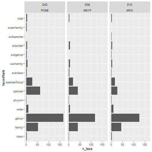
# no. taxa by rank by site

table_observation_cleaned %>% 
  group_by(domainID, siteID, taxonRank) %>%
  summarize(
    n_taxa = acceptedTaxonID %>% 
        unique() %>% length()) %>%
  ggplot(aes(n_taxa, taxonRank)) +
  facet_wrap(~ domainID + siteID) +
  geom_col()

# library(scales)

# sum densities by order for each sampleID

table_observation_by_order <- 
    table_observation_cleaned %>% 
    filter(!is.na(order)) %>%
    group_by(domainID, siteID, year, 
             eventID, sampleID, habitatType, order) %>%
    summarize(order_dens = sum(inv_dens, na.rm = TRUE))

  

  

# rank occurrence by order

table_observation_by_order %>% head()

## # A tibble: 6 × 8
## # Groups:   domainID, siteID, year, eventID, sampleID, habitatType [1]
##   domainID siteID  year eventID       sampleID               habitatType order            order_dens
##   <chr>    <chr>  <dbl> <chr>         <chr>                  <chr>       <chr>                 <dbl>
## 1 D02      POSE    2014 POSE.20140722 POSE.20140722.SURBER.1 riffle      Branchiobdellida      516. 
## 2 D02      POSE    2014 POSE.20140722 POSE.20140722.SURBER.1 riffle      Coleoptera            516. 
## 3 D02      POSE    2014 POSE.20140722 POSE.20140722.SURBER.1 riffle      Decapoda               86.0
## 4 D02      POSE    2014 POSE.20140722 POSE.20140722.SURBER.1 riffle      Diptera              5419. 
## 5 D02      POSE    2014 POSE.20140722 POSE.20140722.SURBER.1 riffle      Ephemeroptera        5301. 
## 6 D02      POSE    2014 POSE.20140722 POSE.20140722.SURBER.1 riffle      Megaloptera           387.

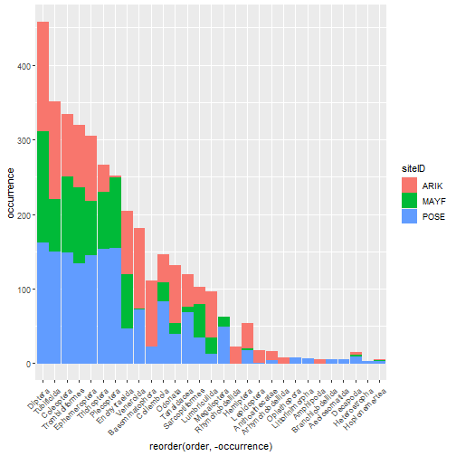
# stacked rank occurrence plot

table_observation_by_order %>%
  group_by(order, siteID) %>%
  summarize(
    occurrence = (order_dens > 0) %>% sum()) %>%
    ggplot(aes(
        x = reorder(order, -occurrence), 
        y = occurrence,
        color = siteID,
        fill = siteID)) +
    geom_col() +
    theme(axis.text.x = 
              element_text(angle = 45, hjust = 1))

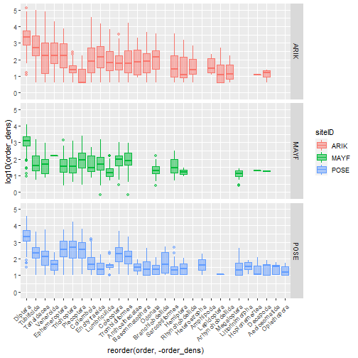
# faceted densities plot

table_observation_by_order %>%
  ggplot(aes(
    x = reorder(order, -order_dens), 
    y = log10(order_dens),
    color = siteID,
    fill = siteID)) +
  geom_boxplot(alpha = .5) +
  facet_grid(siteID ~ .) +
  theme(axis.text.x = 
            element_text(angle = 45, hjust = 1))

Making Data 'wide'

For the next process, we will need to make our data table in the 'wide' format.

# select only site by species density info and remove duplicate records

table_sample_by_taxon_density_long <- table_observation_cleaned %>%
  select(sampleID, acceptedTaxonID, inv_dens) %>%
  distinct() %>%
  filter(!is.na(inv_dens))



# table_sample_by_taxon_density_long %>% nrow()

# table_sample_by_taxon_density_long %>% distinct() %>% nrow()







# pivot to wide format, sum multiple counts per sampleID

table_sample_by_taxon_density_wide <- table_sample_by_taxon_density_long %>%
  tidyr::pivot_wider(id_cols = sampleID, 
                     names_from = acceptedTaxonID,
                     values_from = inv_dens,
                     values_fill = list(inv_dens = 0),
                     values_fn = list(inv_dens = sum)) %>%
  column_to_rownames(var = "sampleID") 



# check col and row sums -- mins should all be > 0

colSums(table_sample_by_taxon_density_wide) %>% min()

## [1] 12

rowSums(table_sample_by_taxon_density_wide) %>% min()

## [1] 25.55004

Multiscale Biodiversity

Reference: Jost, L. 2007. Partitioning diversity into independent alpha and beta components. Ecology 88:2427–2439. https://doi.org/10.1890/06-1736.1.

These metrics are based on Robert Whittaker's multiplicative diversity where

• gamma is regional biodiversity
• alpha is local biodiversity (e.g., the mean diversity at a patch)
• and beta diversity is a measure of among-patch variability in community composition.

Beta could be interpreted as the number of "distinct" communities present within the region.

The relationship among alpha, beta, and gamma diversity is: beta = gamma / alpha

The influence of relative abundances over the calculation of alpha, beta, and gamma diversity metrics is determined by the coefficient q. The coefficient "q" determines the "order" of the diversity metric, where q = 0 provides diversity measures based on richness, and higher orders of q give more weight to taxa that have higher abundances in the data. Order q = 1 is related to Shannon diveristy metrics, and order q = 2 is related to Simpson diversity metrics.

Alpha diversity is average local richness.

Order q = 0 alpha diversity calculated for our dataset returns a mean local richness (i.e., species counts) of ~30 taxa per sample across the entire data set.

# Here we use vegan::renyi to calculate Hill numbers

# If hill = FALSE, the function returns an entropy

# If hill = TRUE, the function returns the exponentiated

# entropy. In other words:

# exp(renyi entropy) = Hill number = "species equivalent"



# Note that for this function, the "scales" argument 

# determines the order of q used in the calculation



table_sample_by_taxon_density_wide %>%
  vegan::renyi(scales = 0, hill = TRUE) %>%
  mean()

## [1] 30.17635

Comparing alpha diversity calculated using different orders:

Order q = 1 alpha diversity returns mean number of "species equivalents" per sample in the data set. This approach incorporates evenness because when abundances are more even across taxa, taxa are weighted more equally toward counting as a "species equivalent". For example, if you have a sample with 100 individuals, spread across 10 species, and each species is represented by 10 individuals, the number of order q = 1 species equivalents will equal the richness (10).

Alternatively, if 90 of the 100 individuals in the sample are one species, and the other 10 individuals are spread across the other 9 species, there will only be 1.72 order q = 1 species equivalents, whereas, there are still 10 species in the sample.

# even distribution, orders q = 0 and q = 1 for 10 taxa

vegan::renyi(
  c(spp.a = 10, spp.b = 10, spp.c = 10, 
    spp.d = 10, spp.e = 10, spp.f = 10, 
    spp.g = 10, spp.h = 10, spp.i = 10, 
    spp.j = 10),
  hill = TRUE,
  scales = c(0, 1))

##  0  1 
## 10 10 
## attr(,"class")
## [1] "renyi"   "numeric"

# uneven distribution, orders q = 0 and q = 1 for 10 taxa

vegan::renyi(
  c(spp.a = 90, spp.b = 2, spp.c = 1, 
    spp.d = 1, spp.e = 1, spp.f = 1, 
    spp.g = 1, spp.h = 1, spp.i = 1, 
    spp.j = 1),
  hill = TRUE,
  scales = c(0, 1)) 

##         0         1 
## 10.000000  1.718546 
## attr(,"class")
## [1] "renyi"   "numeric"

Comparing orders of q for NEON data

Let's compare the different orders q = 0, 1, and 2 measures of alpha diversity across the samples collected from ARIK, POSE, and MAYF.

# Nest data by siteID

data_nested_by_siteID <- table_sample_by_taxon_density_wide %>%
  tibble::rownames_to_column("sampleID") %>%
  left_join(table_sample_info %>% 
                select(sampleID, siteID)) %>%
  tibble::column_to_rownames("sampleID") %>%
  nest(data = -siteID)



data_nested_by_siteID$data[[1]] %>%
  vegan::renyi(scales = 0, hill = TRUE) %>%
  mean()

## [1] 25.23226

# apply the calculation by site for alpha diversity

# for each order of q

data_nested_by_siteID %>% mutate(
  alpha_q0 = purrr::map_dbl(
    .x = data,
    .f = ~ vegan::renyi(x = .,
                        hill = TRUE, 
                        scales = 0) %>% mean()),
  alpha_q1 = purrr::map_dbl(
    .x = data,
    .f = ~ vegan::renyi(x = .,
                        hill = TRUE, 
                        scales = 1) %>% mean()),
  alpha_q2 = purrr::map_dbl(
    .x = data,
    .f = ~ vegan::renyi(x = .,
                        hill = TRUE, 
                        scales = 2) %>% mean())
  )

## # A tibble: 3 × 5
##   siteID data                 alpha_q0 alpha_q1 alpha_q2
##   <chr>  <list>                  <dbl>    <dbl>    <dbl>
## 1 ARIK   <tibble [155 × 469]>     25.2     10.5     6.73
## 2 MAYF   <tibble [157 × 469]>     22.1     12.0     8.21
## 3 POSE   <tibble [170 × 469]>     42.1     20.7    12.9

# Note that POSE has the highest mean alpha diversity







# To calculate gamma diversity at the site scale,

# calculate the column means and then calculate 

# the renyi entropy and Hill number

# Here we are only calcuating order 

# q = 0 gamma diversity

data_nested_by_siteID %>% mutate(
  gamma_q0 = purrr::map_dbl(
    .x = data,
    .f = ~ vegan::renyi(x = colMeans(.),
                        hill = TRUE, 
                        scales = 0)))

## # A tibble: 3 × 3
##   siteID data                 gamma_q0
##   <chr>  <list>                  <dbl>
## 1 ARIK   <tibble [155 × 469]>     252 
## 2 MAYF   <tibble [157 × 469]>     243 
## 3 POSE   <tibble [170 × 469]>     343.

# Note that POSE has the highest gamma diversity







# Now calculate alpha, beta, and gamma using orders 0 and 1 

# for each siteID

diversity_partitioning_results <- 
  data_nested_by_siteID %>% 
  mutate(
    n_samples = purrr::map_int(data, ~ nrow(.)),
    alpha_q0 = purrr::map_dbl(
      .x = data,
      .f = ~ vegan::renyi(x = .,
                          hill = TRUE, 
                          scales = 0) %>% mean()),
    alpha_q1 = purrr::map_dbl(
      .x = data,
      .f = ~ vegan::renyi(x = .,
                          hill = TRUE, 
                          scales = 1) %>% mean()),
    gamma_q0 = purrr::map_dbl(
      .x = data,
      .f = ~ vegan::renyi(x = colMeans(.),
                          hill = TRUE, 
                          scales = 0)),
    gamma_q1 = purrr::map_dbl(
      .x = data,
      .f = ~ vegan::renyi(x = colMeans(.),
                          hill = TRUE, 
                          scales = 1)),
    beta_q0 = gamma_q0 / alpha_q0,
    beta_q1 = gamma_q1 / alpha_q1)





diversity_partitioning_results %>% 
  select(-data) %>% as.data.frame() %>% print()

##   siteID n_samples alpha_q0 alpha_q1 gamma_q0  gamma_q1   beta_q0  beta_q1
## 1   ARIK       155 25.23226 10.54023      252  36.59410  9.987216 3.471851
## 2   MAYF       157 22.13376 12.01255      243  67.12029 10.978705 5.587514
## 3   POSE       170 42.11176 20.70407      343 100.48550  8.144992 4.853419

Using NMDS to ordinate samples

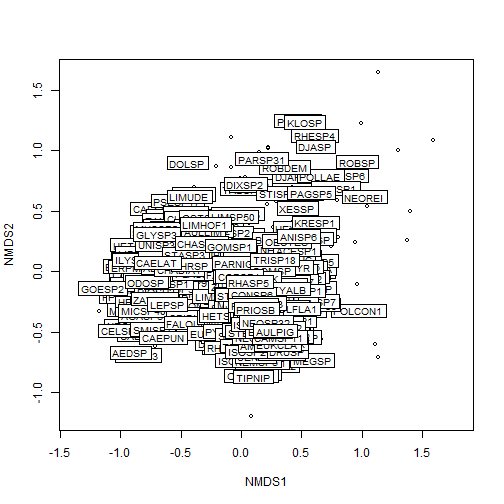
Finally, we will use Nonmetric Multidimensional Scaling (NMDS) to ordinate samples as shown below:

# create ordination using NMDS

my_nmds_result <- table_sample_by_taxon_density_wide %>% vegan::metaMDS()

## Square root transformation
## Wisconsin double standardization
## Run 0 stress 0.2294109 
## Run 1 stress 0.2434733 
## Run 2 stress 0.2333922 
## Run 3 stress 0.2295899 
## ... Procrustes: rmse 0.009527262  max resid 0.1652604 
## Run 4 stress 0.2324826 
## Run 5 stress 0.243147 
## Run 6 stress 0.2365832 
## Run 7 stress 0.2488192 
## Run 8 stress 0.2364006 
## Run 9 stress 0.2527803 
## Run 10 stress 0.241648 
## Run 11 stress 0.2357162 
## Run 12 stress 0.2381212 
## Run 13 stress 0.2371189 
## Run 14 stress 0.2509742 
## Run 15 stress 0.2538595 
## Run 16 stress 0.2319501 
## Run 17 stress 0.2413884 
## Run 18 stress 0.2335127 
## Run 19 stress 0.2389742 
## Run 20 stress 0.2388227 
## *** Best solution was not repeated -- monoMDS stopping criteria:
##      1: no. of iterations >= maxit
##     17: stress ratio > sratmax
##      2: scale factor of the gradient < sfgrmin

# plot stress

my_nmds_result$stress

## [1] 0.2294109

p1 <- vegan::ordiplot(my_nmds_result)

vegan::ordilabel(p1, "species")

# merge NMDS scores with sampleID information for plotting

nmds_scores <- my_nmds_result %>% 
  vegan::scores() %>%
  .[["sites"]] %>%
  as.data.frame() %>%
  tibble::rownames_to_column("sampleID") %>%
  left_join(table_sample_info)





# # How I determined the outlier(s)

nmds_scores %>% arrange(desc(NMDS1)) %>% head()

##               sampleID    NMDS1      NMDS2 domainID siteID  namedLocation         collectDate       eventID year
## 1 MAYF.20190311.CORE.2 1.538203  1.1079007      D08   MAYF MAYF.AOS.reach 2019-03-11 15:00:00 MAYF.20190311 2019
## 2 MAYF.20201117.CORE.2 1.320586  0.5034843      D08   MAYF MAYF.AOS.reach 2020-11-17 16:33:00 MAYF.20201117 2020
## 3 MAYF.20180726.CORE.2 1.310929  0.3070852      D08   MAYF MAYF.AOS.reach 2018-07-26 14:17:00 MAYF.20180726 2018
## 4 MAYF.20190311.CORE.1 1.244127  1.0084388      D08   MAYF MAYF.AOS.reach 2019-03-11 15:00:00 MAYF.20190311 2019
## 5 MAYF.20170314.CORE.1 1.099424  1.6634308      D08   MAYF MAYF.AOS.reach 2017-03-14 14:11:00 MAYF.20170314 2017
## 6 MAYF.20150324.SNAG.3 1.098810 -0.5347298      D08   MAYF MAYF.AOS.reach 2015-03-24 17:15:00 MAYF.20150324 2015
##   habitatType samplerType benthicArea          inv_dens_unit
## 1         run        core       0.006 count per square meter
## 2         run        core       0.006 count per square meter
## 3         run        core       0.006 count per square meter
## 4         run        core       0.006 count per square meter
## 5         run        core       0.006 count per square meter
## 6         run        snag       0.076 count per square meter

nmds_scores %>% arrange(desc(NMDS1)) %>% tail()

##                    sampleID      NMDS1       NMDS2 domainID siteID  namedLocation         collectDate       eventID year
## 477 ARIK.20160919.KICKNET.5 -0.8135799 -0.26195623      D10   ARIK ARIK.AOS.reach 2016-09-19 22:06:00 ARIK.20160919 2016
## 478 ARIK.20160919.KICKNET.1 -0.8440059  0.24971446      D10   ARIK ARIK.AOS.reach 2016-09-19 22:06:00 ARIK.20160919 2016
## 479    ARIK.20150714.CORE.3 -0.8510254 -0.02350526      D10   ARIK ARIK.AOS.reach 2015-07-14 14:55:00 ARIK.20150714 2015
## 480    ARIK.20150714.CORE.2 -1.0051934 -0.02660317      D10   ARIK ARIK.AOS.reach 2015-07-14 14:55:00 ARIK.20150714 2015
## 481 ARIK.20160919.KICKNET.4 -1.0464997 -0.18522871      D10   ARIK ARIK.AOS.reach 2016-09-19 22:06:00 ARIK.20160919 2016
## 482    ARIK.20160331.CORE.3 -1.1247964 -0.34914016      D10   ARIK ARIK.AOS.reach 2016-03-31 15:41:00 ARIK.20160331 2016
##     habitatType     samplerType benthicArea          inv_dens_unit
## 477         run modifiedKicknet       0.250 count per square meter
## 478         run modifiedKicknet       0.250 count per square meter
## 479        pool            core       0.006 count per square meter
## 480        pool            core       0.006 count per square meter
## 481         run modifiedKicknet       0.250 count per square meter
## 482        pool            core       0.006 count per square meter

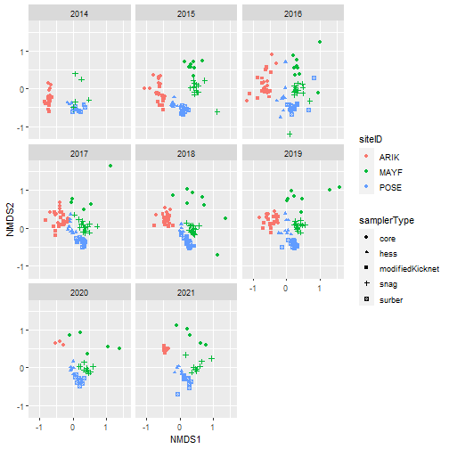
# Plot samples in community composition space by year

nmds_scores %>%
  ggplot(aes(NMDS1, NMDS2, color = siteID, 
             shape = samplerType)) +
  geom_point() +
  facet_wrap(~ as.factor(year))

# Plot samples in community composition space

# facet by siteID and habitat type

# color by year

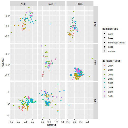
nmds_scores %>%
  ggplot(aes(NMDS1, NMDS2, color = as.factor(year), 
             shape = samplerType)) +
  geom_point() +
  facet_grid(habitatType ~ siteID, scales = "free")