Download and work with NEON Aquatic Instrument Data

This tutorial covers downloading NEON Aquatic Instrument System (AIS) data using the neonUtilities R package, as well as basic instruction in exploring and working with the downloaded data. You will learn how to navigate data documentation, separate data using the horizontalPosition variable, and interpret quality flags.

Download Files and Load Directly to R: loadByProduct()

The most popular function in neonUtilities is loadByProduct(). This function downloads data from the NEON API, merges the site-by-month files, and loads the resulting data tables into the R environment, assigning each data type to the appropriate R class. This is a popular choice because it ensures you're always working with the most up-to-date data, and it ends with ready-to-use tables in R. However, if you use it in a workflow you run repeatedly, keep in mind it will re-download the data every time.

Before we get the NEON data, we need to install (if not already done) and load the neonUtilities R package, as well as other packages we will use in the analysis.

# Install neonUtilities package if you have not yet.

install.packages("neonUtilities")

install.packages("ggplot2")


# Set global option to NOT convert all character variables to factors

options(stringsAsFactors=F)



# Load required packages

library(neonUtilities)

library(ggplot2)

The inputs to loadByProduct() control which data to download and how to manage the processing. The following are frequently used inputs:

• dpID: the NEON data product ID, e.g. "DP1.20288.001"
• site: 4-letter NEON site code, e.g. "ARIK", or vector of of multiple sites, e.g. "c("MART","ARIK","BARC")". Defaults to "all", meaning all sites.
• startdate and enddate: start and end dates for period to be downloaded in the form YYYY-MM, e.g. "2017-06". Defaults to NA, meaning all available data.
• package: specifies either "basic" or "expanded" data package. Expanded data packages generally include additional information about data quality, such as individual quality flag test results. Not every NEON data product has an expanded package; if the expanded package is requested but there isn't one, the basic package will be downloaded.
• release: release version to be downloaded, e.g. "RELEASE-2023". To download the most recent release as well as provisional data (not yet QAQC'ed and included in a versioned release) use "current".
• savepath: the file path you want to download to; defaults to the working directory.
• check.size: T or F; should the function pause before downloading data and warn you about the size of your download? Defaults to T; if you are using this function within a script or batch process you will want to set this to F.
• token: this allows you to input your NEON API token to obtain faster downloads.

Learn more about NEON API tokens in the Using an API Token when Accessing NEON Data with neonUtilities tutorial.

There are additional inputs you can learn about in the Use the neonUtilities R Package to Access NEON Data tutorial.

The dpID is the data product identifier of the data you want to download. The DPID can be found on the Explore Data Products page.

It will be in the form DP#.#####.###. For this tutorial, we'll use NEON's most commonly downloaded AIS data products, Water quality.

• DP1.20288.001: Water quality

Now it's time to consider the NEON field site of interest. If not specified, the default will download a data product from all sites. The following are 4-letter site codes for NEON's 34 aquatics sites as of 2020:

• ARIK = Arikaree River CO
• BARC = Barco Lake FL
• BIGC = Upper Big Creek CA
• BLDE = Black Deer Creek WY
• BLUE = Blue River OK
• BLWA = Black Warrior River AL
• CARI = Caribou Creek AK
• COMO = Como Creek CO
• CRAM = Crampton Lake WI
• CUPE = Rio Cupeyes PR
• FLNT = Flint River GA
• GUIL = Rio Yahuecas PR
• HOPB = Lower Hop Brook MA
• KING = Kings Creek KS
• LECO = LeConte Creek TN
• LEWI = Lewis Run VA
• LIRO = Little Rock Lake WI
• MART = Martha Creek WA
• MAYF = Mayfield Creek AL
• MCDI = McDiffett Creek KS
• MCRA = McRae Creek OR
• OKSR = Oksrukuyik Creek AK
• POSE = Posey Creek VA
• PRIN = Pringle Creek TX
• PRLA = Prairie Lake ND
• PRPO = Prairie Pothole ND
• REDB = Red Butte Creek UT
• SUGG = Suggs Lake FL
• SYCA = Sycamore Creek AZ
• TECR = Teakettle Creek CA
• TOMB = Lower Tombigbee River AL
• TOOK = Toolik Lake AK
• WALK = Walker Branch TN
• WLOU = West St Louis Creek CO

In this exercise, we will use data from only one NEON field site, Pringle Creek, TX from February 2020. Because we want to examine individual quality flags we will download the expanded package. We want the most current release. Finally, since we are only downloading one site-month of data we do not need to check the file size, but for larger downloads this is advisable.

# download data of interest - Water Quality

waq <- loadByProduct(dpID="DP1.20288.001", site="PRIN", 
                     startdate="2020-02", enddate="2020-02", 
                     package="expanded", release="current", 
                     check.size = F)

Files Associated with Downloads

The data we've downloaded comes as a list of objects.

# view all components of the list

names(waq)

##  [1] "ais_maintenance"             "ais_multisondeCleanCal"      "categoricalCodes_20288"      "citation_20288_RELEASE-2023" "issueLog_20288"             
##  [6] "readme_20288"                "science_review_flags_20288"  "sensor_positions_20288"      "variables_20288"             "waq_instantaneous"

We can see that there are multiple objects in the downloaded water quality data. One dataframe of data (waq_instantaneous) and multiple metadata files.

If you'd like you can use the $ operator to assign an object from an item in the list. If you prefer to extract each table from the list and work with it as independent objects, which we will do, you can use the list2env() function.

# unlist the variables and add to the global environment

list2env(waq, .GlobalEnv)

So what exactly are these files and why would you want to use them?

• data file(s): There will always be one or more dataframes that include the primary data of the data product you downloaded. Multiple dataframes are available when there are related datatables for a single data product. For example, some data products are averaged at multiple intervals (e.x. 5-min averages and 30-min averages).
• sensor_postions_#####: this file contains information about the coordinates of each sensor, relative to a reference location.
• variables_#####: this file contains all the variables found in the associated data table(s). This includes full definitions, units, and other important information.
• readme_#####: The readme file, with the corresponding 5 digits from the data product number, provides you with important information relevant to the data product.
• maintenance record(s): Some data products come with maintenance records with information related to cleaning and calibration of sensors.

Let's take a look at a couple of these.

# which sensor locations exist in the water quality dataset we just downloaded?

View(waq_instantaneous)

View(sensor_positions_20288)

View(variables_20288)

Data versioning and citation

Let's check what release(s) our data is from (remember we used "current"). Each static data release has a unique DOI that should be cited. If any provisional data is included it should also be cited (including download date), and archived because provisional data is non-static.

# which release is the data from?

unique(waq_instantaneous$release)

## [1] "RELEASE-2023"

Learn more about data versioning and appropriately reuse of NEON data on the NEON Data Guidelines and Policy page.

Data from Different Sensor Locations

NEON often collects the same type of data from sensors in different locations. These data are delivered together but you will frequently want to plot the data separately or only include data from one sensor in your analysis. NEON uses the horizontalPosition variable in the data tables to describe which sensor data is collected from. The horizontalPosition (HOR) is always a three digit number. Non-shoreline HOR examples as of 2024 at AIS sites include:

• 101: stream sensors located at the upstream station on a monopod mount,
• 111: stream sensors located at the upstream station on an overhead cable mount,
• 131: stream sensors located at the upstream station on a stand alone pressure transducer mount,
• 102: stream sensors located at the downstream station on a monopod mount,
• 112: stream sensors located at the downstream station on an overhead cable mount
• 132: stream sensors located at the downstream station on a stand alone pressure transducer mount,
• 110: stream pressure transducers mounted directly to a staff gauge.
• 103: sensors mounted on buoys in lakes or rivers
• 130, 140, 150, 160, 180 and and 190: sensors mounted in the littoral zone of lakes

Note that data is also collected at different vertical positions (VER) at lake and river sites. This example is from a wadeable stream site with only a single VER.

You'll frequently want to know which sensor locations are represented in your data. We can do this by looking for the unique() position designations in horizontalPostions.

# which sensor locations exist in the water quality dataset we just downloaded?

unique(waq_instantaneous$horizontalPosition)

## [1] "101" "102"

We can see that there are two water quality horizontal positions present in the data, upstream and downstream. As the HOR of sensors can change at sites over time, as well as the physical location corresponding to a particular HOR, it is a good idea to review the sensor_positions file when you're adding in new sites or a new date range to your analyses.

We can use this information to split water quality data into the two different sensor set locations: upstream and the downstream.

# Split data into separate dataframes by upstream/downstream locations.

waq_up <- 
  waq_instantaneous[(waq_instantaneous$horizontalPosition=="101"),]

waq_down <- 
  waq_instantaneous[(waq_instantaneous$horizontalPosition=="102"),]

Plot Data

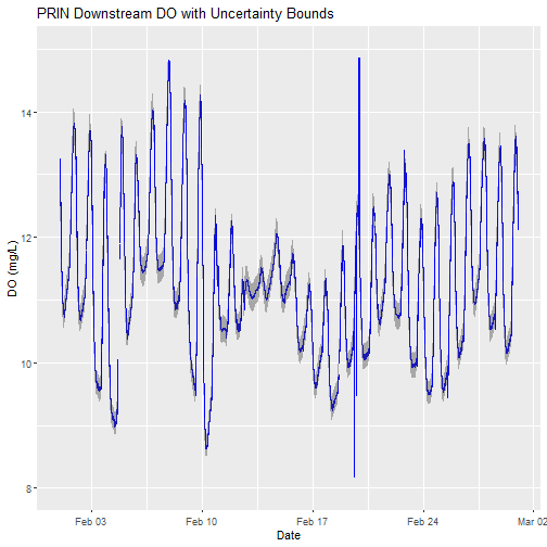
Now that we have our data separated into the upstream and downstream data, let's plot Dissolved Oxygen from the downstream sensor. NEON also includes uncertainty estimates for most of its measurements. Let's include those in the plot as well.

First, let's identify the column names important for plotting - time and dissolved oxygen data:

# One option is to view column names in the data frame

colnames(waq_instantaneous)

##   [1] "domainID"                      "siteID"                        "horizontalPosition"            "verticalPosition"             
##   [5] "startDateTime"                 "endDateTime"                   "sensorDepth"                   "sensorDepthExpUncert"         
##   [9] "sensorDepthRangeQF"            "sensorDepthNullQF"             "sensorDepthGapQF"              "sensorDepthValidCalQF"        
##  [13] "sensorDepthSuspectCalQF"       "sensorDepthPersistQF"          "sensorDepthAlphaQF"            "sensorDepthBetaQF"            
##  [17] "sensorDepthFinalQF"            "sensorDepthFinalQFSciRvw"      "specificConductance"           "specificConductanceExpUncert" 
##  [21] "specificConductanceRangeQF"    "specificConductanceStepQF"     "specificConductanceNullQF"     "specificConductanceGapQF"     
##  [25] "specificConductanceSpikeQF"    "specificConductanceValidCalQF" "specificCondSuspectCalQF"      "specificConductancePersistQF" 
##  [29] "specificConductanceAlphaQF"    "specificConductanceBetaQF"     "specificCondFinalQF"           "specificCondFinalQFSciRvw"    
##  [33] "dissolvedOxygen"               "dissolvedOxygenExpUncert"      "dissolvedOxygenRangeQF"        "dissolvedOxygenStepQF"        
##  [37] "dissolvedOxygenNullQF"         "dissolvedOxygenGapQF"          "dissolvedOxygenSpikeQF"        "dissolvedOxygenValidCalQF"    
##  [41] "dissolvedOxygenSuspectCalQF"   "dissolvedOxygenPersistenceQF"  "dissolvedOxygenAlphaQF"        "dissolvedOxygenBetaQF"        
##  [45] "dissolvedOxygenFinalQF"        "dissolvedOxygenFinalQFSciRvw"  "seaLevelDissolvedOxygenSat"    "seaLevelDOSatExpUncert"       
##  [49] "seaLevelDOSatRangeQF"          "seaLevelDOSatStepQF"           "seaLevelDOSatNullQF"           "seaLevelDOSatGapQF"           
##  [53] "seaLevelDOSatSpikeQF"          "seaLevelDOSatValidCalQF"       "seaLevelDOSatSuspectCalQF"     "seaLevelDOSatPersistQF"       
##  [57] "seaLevelDOSatAlphaQF"          "seaLevelDOSatBetaQF"           "seaLevelDOSatFinalQF"          "seaLevelDOSatFinalQFSciRvw"   
##  [61] "localDissolvedOxygenSat"       "localDOSatExpUncert"           "localDOSatRangeQF"             "localDOSatStepQF"             
##  [65] "localDOSatNullQF"              "localDOSatGapQF"               "localDOSatSpikeQF"             "localDOSatValidCalQF"         
##  [69] "localDOSatSuspectCalQF"        "localDOSatPersistQF"           "localDOSatAlphaQF"             "localDOSatBetaQF"             
##  [73] "localDOSatFinalQF"             "localDOSatFinalQFSciRvw"       "pH"                            "pHExpUncert"                  
##  [77] "pHRangeQF"                     "pHStepQF"                      "pHNullQF"                      "pHGapQF"                      
##  [81] "pHSpikeQF"                     "pHValidCalQF"                  "pHSuspectCalQF"                "pHPersistenceQF"              
##  [85] "pHAlphaQF"                     "pHBetaQF"                      "pHFinalQF"                     "pHFinalQFSciRvw"              
##  [89] "chlorophyll"                   "chlorophyllExpUncert"          "chlorophyllRangeQF"            "chlorophyllStepQF"            
##  [93] "chlorophyllNullQF"             "chlorophyllGapQF"              "chlorophyllSpikeQF"            "chlorophyllValidCalQF"        
##  [97] "chlorophyllSuspectCalQF"       "chlorophyllPersistenceQF"      "chlorophyllAlphaQF"            "chlorophyllBetaQF"            
## [101] "chlorophyllFinalQF"            "chlorophyllFinalQFSciRvw"      "chlaRelativeFluorescence"      "chlaRelFluoroExpUncert"       
## [105] "chlaRelFluoroRangeQF"          "chlaRelFluoroStepQF"           "chlaRelFluoroNullQF"           "chlaRelFluoroGapQF"           
## [109] "chlaRelFluoroSpikeQF"          "chlaRelFluoroValidCalQF"       "chlaRelFluoroSuspectCalQF"     "chlaRelFluoroPersistenceQF"   
## [113] "chlaRelFluoroAlphaQF"          "chlaRelFluoroBetaQF"           "chlaRelFluoroFinalQF"          "chlaRelFluoroFinalQFSciRvw"   
## [117] "turbidity"                     "turbidityExpUncert"            "turbidityRangeQF"              "turbidityStepQF"              
## [121] "turbidityNullQF"               "turbidityGapQF"                "turbiditySpikeQF"              "turbidityValidCalQF"          
## [125] "turbiditySuspectCalQF"         "turbidityPersistenceQF"        "turbidityAlphaQF"              "turbidityBetaQF"              
## [129] "turbidityFinalQF"              "turbidityFinalQFSciRvw"        "fDOM"                          "rawCalibratedfDOM"            
## [133] "fDOMExpUncert"                 "fDOMRangeQF"                   "fDOMStepQF"                    "fDOMNullQF"                   
## [137] "fDOMGapQF"                     "fDOMSpikeQF"                   "fDOMValidCalQF"                "fDOMSuspectCalQF"             
## [141] "fDOMPersistenceQF"             "fDOMAlphaQF"                   "fDOMBetaQF"                    "fDOMTempQF"                   
## [145] "fDOMAbsQF"                     "fDOMFinalQF"                   "fDOMFinalQFSciRvw"             "buoyNAFlag"                   
## [149] "spectrumCount"                 "publicationDate"               "release"


# Alternatively, view the variables object corresponding to the data product for more information

View(variables_20288)

Quite a few columns in the water quality data product!

The time column we'll consider for instrumented systems is endDateTime. Timestamp column choice (e.g. start or end) matters for time-aggregated datasets, but should not matter for instantaneous data such as water quality. When interpreting data, keep in mind NEON timestamps are always in UTC.

The data columns we would like to plot are dissolvedOxygen and dissolvedOxygenExpUncert.

# plot

doPlot <- ggplot() +
	geom_line(data = waq_down,aes(endDateTime, dissolvedOxygen),na.rm=TRUE, color="blue") +
  geom_ribbon(data=waq_down,aes(x=endDateTime, 
                  ymin = (dissolvedOxygen - dissolvedOxygenExpUncert), 
                  ymax = (dissolvedOxygen + dissolvedOxygenExpUncert)), 
              alpha = 0.4, fill = "grey25") +
	ylim(8, 15) + ylab("DO (mg/L)") + xlab("Date") + ggtitle("PRIN Downstream DO with Uncertainty Bounds") 



doPlot

Examine Quality Flagged Data

Data product quality flags fall under two distinct types:

• Automated quality flags, e.g. range, spike, step, null
• Manual science review quality flag

In instantaneous data such as water quality, the quality flag columns are denoted with "QF". In time-averaged data, most quality flags have been aggregated into quality metrics, with column names denoted with "QM" representing the fraction of flagged points within the time averaging window.

waq_qf_names <- names(waq_down)[grep("QF", names(waq_down))]



print(paste0("Total columns in DP1.20288.001 expanded package = ", 
             as.character(length(waq_qf_names))))

## [1] "Total columns in DP1.20288.001 expanded package = 120"

# Let's just look at those corresponding to dissolvedOxygen.

# We need to remove those associated with dissolvedOxygenSaturation.

do_qf_names <- waq_qf_names[grep("dissolvedOxygen",waq_qf_names)]

do_qf_names <- do_qf_names[grep("dissolvedOxygenSat",do_qf_names,invert=T)]



print("dissolvedOxygen columns in DP1.20288.001 expanded package:")

## [1] "dissolvedOxygen columns in DP1.20288.001 expanded package:"

print(do_qf_names)

##  [1] "dissolvedOxygenRangeQF"       "dissolvedOxygenStepQF"        "dissolvedOxygenNullQF"        "dissolvedOxygenGapQF"        
##  [5] "dissolvedOxygenSpikeQF"       "dissolvedOxygenValidCalQF"    "dissolvedOxygenSuspectCalQF"  "dissolvedOxygenPersistenceQF"
##  [9] "dissolvedOxygenAlphaQF"       "dissolvedOxygenBetaQF"        "dissolvedOxygenFinalQF"       "dissolvedOxygenFinalQFSciRvw"

A quality flag (QF) of 0 indicates a pass, 1 indicates a fail, and -1 indicates a test that could not be performed. For example, a range test cannot be performed on missing measurements.

Detailed quality flags test results are all available in the package = 'expanded' setting we specified when calling neonUtilities::loadByProduct(). If we had specified package = 'basic', we wouldn't be able to investigate the detail in the type of data flag thrown. We would only see the FinalQF columns.

The AlphaQF and BetaQF represent aggregated results of various QF tests, and vary by a data product's algorithm. In most cases, an observation's AlphaQF = 1 indicates whether or not at least one QF was set to a value of 1, and an observation's BetaQF = 1 indicates whether or not at least one QF was set to value of -1.

Let's consider what types of quality flags were thrown.

for(col_nam in do_qf_names){
  print(paste0(col_nam, " unique values: ", 
               paste0(unique(waq_down[,col_nam]), 
                      collapse = ", ")))
}

## [1] "dissolvedOxygenRangeQF unique values: 0, -1"
## [1] "dissolvedOxygenStepQF unique values: 0, -1, 1"
## [1] "dissolvedOxygenNullQF unique values: 0, 1"
## [1] "dissolvedOxygenGapQF unique values: 0, 1"
## [1] "dissolvedOxygenSpikeQF unique values: 0, -1"
## [1] "dissolvedOxygenValidCalQF unique values: 0"
## [1] "dissolvedOxygenSuspectCalQF unique values: 0"
## [1] "dissolvedOxygenPersistenceQF unique values: 0"
## [1] "dissolvedOxygenAlphaQF unique values: 0, 1"
## [1] "dissolvedOxygenBetaQF unique values: 0, 1"
## [1] "dissolvedOxygenFinalQF unique values: 0, 1"
## [1] "dissolvedOxygenFinalQFSciRvw unique values: NA"

QF values generally mean the following:

• 0: Quality test passed
• 1: Quality test failed
• -1: Quality test could not be run

Now let's consider the total number of flags generated for each quality test:

# Loop across the QF column names. 

#  Within each column, count the number of rows that equal '1'.

print("FLAG TEST - COUNT")

## [1] "FLAG TEST - COUNT"

for (col_nam in do_qf_names){
  totl_qf_in_col <- length(which(waq_down[,col_nam] == 1))
  print(paste0(col_nam,": ",totl_qf_in_col))
}

## [1] "dissolvedOxygenRangeQF: 0"
## [1] "dissolvedOxygenStepQF: 23"
## [1] "dissolvedOxygenNullQF: 224"
## [1] "dissolvedOxygenGapQF: 211"
## [1] "dissolvedOxygenSpikeQF: 0"
## [1] "dissolvedOxygenValidCalQF: 0"
## [1] "dissolvedOxygenSuspectCalQF: 0"
## [1] "dissolvedOxygenPersistenceQF: 0"
## [1] "dissolvedOxygenAlphaQF: 247"
## [1] "dissolvedOxygenBetaQF: 229"
## [1] "dissolvedOxygenFinalQF: 247"
## [1] "dissolvedOxygenFinalQFSciRvw: 0"

print(paste0("Total DO observations: ", nrow(waq_down) ))

## [1] "Total DO observations: 41760"

Above lists the total DO QFs, as well as the total number of observation data points in the data file.

For specific details on the algorithms used to create a data product and its corresponding quality tests, it's best to first check the data product's Algorithm Theoretical Basis Document (ATBD) available for download on the data product's web page.

Are there any manual science review quality flags? If so, the explanation for flagging may also be viewed science_review_flags file that comes with the download.

Note that the automated quality flag algorithms are not perfect, and suspect data points may occasionally pass the quality tests. Other times potentially useful data may get quality flagged. Ultimately it is up to the user to decide which data they are comfortable using, which is why we recommend using the expanded data package to better understand why data are being flagged.

Replot, with quality flags filtered by color

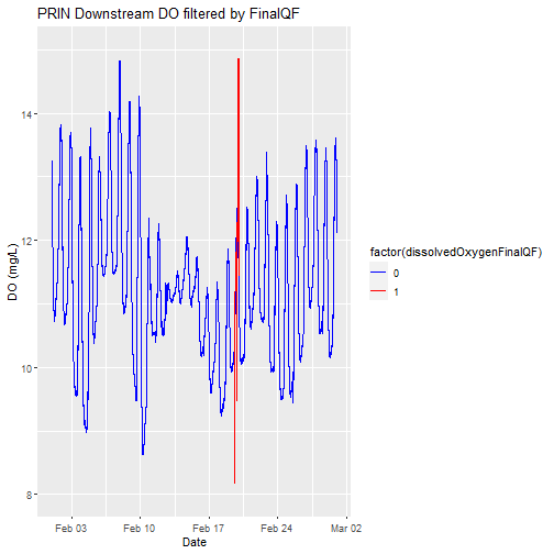
Let's replot the data with any quality flagged measurements set to a different color.

# plot

doPlot <- ggplot() +
	geom_line(data = waq_down, aes(x=endDateTime, y=dissolvedOxygen,
	                 color=factor(dissolvedOxygenFinalQF)), na.rm=TRUE) +
  scale_color_manual(values = c("0" = "blue","1"="red")) +
  ylim(8, 15) + ylab("DO (mg/L)") + xlab("Date") + ggtitle("PRIN Downstream DO filtered by FinalQF") 

  

doPlot

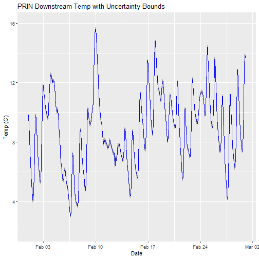
Apply what we've learned Part 1 - Temperature of Surface Water

Applying what we've learned, let's look at a different data product,Temperature of Surface Water (DP1.20053.001). Can you download for the same site and month that we just looked at for water quality?

# download continuous discharge data

csd <- loadByProduct(dpID="DP1.20053.001", site="PRIN", 
                     startdate="2020-02", enddate="2020-02", 
                     package="expanded", release="current", 
                     check.size = F)

list2env(csd,.GlobalEnv)

This data product also comes with sensor_position_#####, variables_#####, readme_#####, and other metadata files. But did you notice anything different about the data file(s)? Temperature of surface water is an averaged data product and comes with both a 5min and 30min data file. Let's use the 30min.

What horizontal positions are present in the data?

# which sensor locations exist in the temperature of surface water dataset?

unique(TSW_30min$horizontalPosition)

## [1] "101" "102"

Let's use the downstream data just like we did for water quality.

# Split data into separate dataframe for downstream location.

tsw_down <- 
  TSW_30min[(TSW_30min$horizontalPosition=="102"),]

Can you remove the quality flagged values?

# remove values with a final quality flag

tsw_down<-tsw_down[(tsw_down$finalQF=="0"),]

Can you plot the data?

# plot

csdPlot <- ggplot() +
	geom_line(data = tsw_down,aes(endDateTime, surfWaterTempMean),na.rm=TRUE, color="blue") +
  geom_ribbon(data=tsw_down,aes(x=endDateTime, 
                  ymin = (surfWaterTempMean-surfWaterTempExpUncert), 
                  ymax = (surfWaterTempMean+surfWaterTempExpUncert)), 
              alpha = 0.4, fill = "grey25") +
	ylim(2, 16) + ylab("Temp (C)") + xlab("Date") + ggtitle("PRIN Downstream Temp with Uncertainty Bounds") 



csdPlot

Apply what we've learned Part 2 - Continuous discharge

Applying what we've learned, let's look at a different data product, Continuous discharge (DP4.00130.001). Can you download for the same site and month that we just looked at for water quality?

# download continuous discharge data

csd <- loadByProduct(dpID="DP4.00130.001", site="PRIN", 
                     startdate="2020-02", enddate="2020-02", 
                     package="expanded", release="current", 
                     check.size = F)

list2env(csd,.GlobalEnv)

Discharge is only measured a a single location in stream sites, so we don't have to worry about horizontal position. Can you remove the quality flagged values?

# remove values with a final quality flag

csd_continuousDischarge<-csd_continuousDischarge[(csd_continuousDischarge$dischargeFinalQF=="0"),]

Can you plot the discharge data?

# plot

csdPlot <- ggplot() +
	geom_line(data = csd_continuousDischarge,aes(endDate, maxpostDischarge),na.rm=TRUE, color="blue") +
  geom_ribbon(data=csd_continuousDischarge,aes(x=endDate, 
                  ymin = (withRemnUncQLower1Std), 
                  ymax = (withRemnUncQUpper1Std)), 
              alpha = 0.4, fill = "grey25") +
	ylim(0, 4000) + ylab("Q (L/s)") + xlab("Date") + ggtitle("PRIN Discharge with Uncertainty Bounds") 



csdPlot

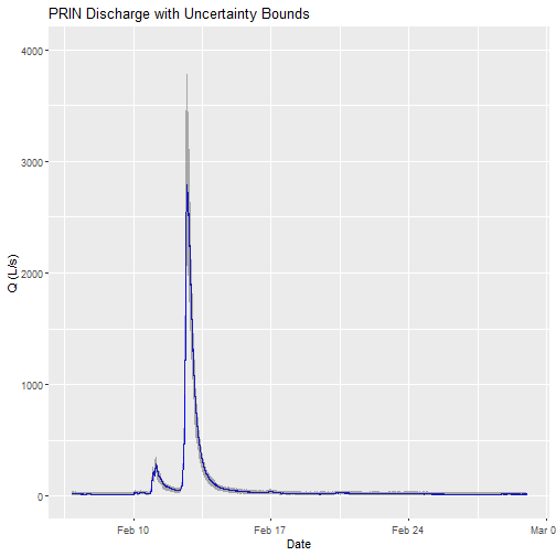
Note: The developers of the Bayesian discharge model used by NEON recommend the maxpostDischarge, which is the mode of the posterior distribution (means and medians are also provided).