Access and Work with NEON Geolocation Data

This tutorial explores NEON geolocation data. The focus is on the locations of NEON observational sampling and sensor data; NEON remote sensing data are inherently spatial and have dedicated tutorials. If you are interested in connecting remote sensing with ground-based measurements, the methods in the vegetation structure and canopy height model tutorial can be generalized to other data products.

In planning your analyses, consider what level of spatial resolution is required. There is no reason to carefully map each measurement if precise spatial locations aren't required to address your hypothesis! For example, if you want to use the Vegetation structure data product to calculate a site-scale estimate of biomass and production, the spatial coordinates of each tree are probably not needed. If you want to explore relationships between vegetation and beetle communities, you will need to identify the sampling plots where NEON measures both beetles and vegetation, but finer-scale coordinates may not be needed. Finally, if you want to relate vegetation measurements to airborne remote sensing data, you will need very accurate coordinates for each measurement on the ground.

Setup R Environment

We'll need several R packages in this tutorial. Install the packages, if not already installed, and load the libraries for each.

# run once to get the package, and re-run if you need to get updates

install.packages("ggplot2")  # plotting

install.packages("neonUtilities")  # work with NEON data

install.packages("neonOS")  # work with NEON observational data

install.packages("devtools")  # to use the install_github() function

devtools::install_github("NEONScience/NEON-geolocation/geoNEON")  # work with NEON spatial data



# run every time you start a script

library(ggplot2)

library(neonUtilities)

library(neonOS)

library(geoNEON)



options(stringsAsFactors=F)

Locations for observational data

Plot level locations

Both aquatic and terrestrial observational data downloads include spatial data in the downloaded files. The spatial data in the aquatic data files are the most precise locations available for the sampling events. The spatial data in the terrestrial data downloads represent the locations of the sampling plots. In some cases, the plot is the most precise location available, but for many terrestrial data products, more precise locations can be calculated for specific sampling events.

Here, we'll download the Vegetation structure (DP1.10098.001) data product, examine the plot location data in the download, then calculate the locations of individual trees. These steps can be extrapolated to other terrestrial observational data products; the specific sampling layout varies from data product to data product, but the methods for working with the data are similar.

First, let's download the vegetation structure data from one site, Wind River Experimental Forest (WREF).

If downloading data using the neonUtilities package is new to you, check out the Download and Explore tutorial.

# load veg structure data

vst <- loadByProduct(dpID="DP1.10098.001", 
                     site="WREF",
                     check.size=F)

Data downloaded this way are stored in R as a large list. For this tutorial, we'll work with the individual dataframes within this large list. Alternatively, each dataframe can be assigned as its own object.

To find the spatial data for any given data product, view the variables files to figure out which data table the spatial data are contained in.

View(vst$variables_10098)

Looking through the variables, we can see that the spatial data (decimalLatitude and decimalLongitude, etc) are in the vst_perplotperyear table. Let's take a look at the table.

View(vst$vst_perplotperyear)

As noted above, the spatial data here are at the plot level; the latitude and longitude represent the centroid of the sampling plot. We can map these plots on the landscape using the easting and northing variables; these are the UTM coordinates. At this site, tower plots are 40 m x 40 m, and distributed plots are 20 m x 20 m; we can use the symbols() function to draw boxes of the correct size.

We'll also use the treesPresent variable to subset to only those plots where trees were found and measured.

# start by subsetting data to plots with trees

vst.trees <- vst$vst_perplotperyear[which(
        vst$vst_perplotperyear$treesPresent=="Y"),]



# make variable for plot sizes

plot.size <- numeric(nrow(vst.trees))



# populate plot sizes in new variable

plot.size[which(vst.trees$plotType=="tower")] <- 40

plot.size[which(vst.trees$plotType=="distributed")] <- 20



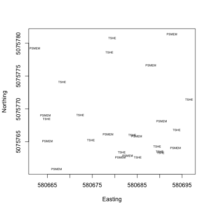
# create map of plots

symbols(vst.trees$easting,
        vst.trees$northing,
        squares=plot.size, inches=F,
        xlab="Easting", ylab="Northing")

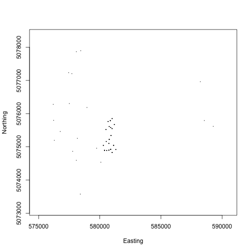
We can see where the plots are located across the landscape, and we can see the denser cluster of plots in the area near the micrometeorology tower.

For many analyses, this level of spatial data may be sufficient. Calculating the precise location of each tree is only required for certain hypotheses; consider whether you need these data when working with a data product with plot-level spatial data.

Looking back at the variables_10098 table, notice that there is a table in this data product called vst_mappingandtagging, suggesting we can find mapping data there. Let's take a look.

View(vst$vst_mappingandtagging)

Here we see data fields for stemDistance and stemAzimuth. Looking back at the variables_10098 file, we see these fields contain the distance and azimuth from a pointID to a specific stem. To calculate the precise coordinates of each tree, we would need to get the locations of the pointIDs, and then adjust the coordinates based on distance and azimuth. The Data Product User Guide describes how to carry out these steps, and can be downloaded from the Data Product Details page.

However, carrying out these calculations yourself is not the only option! The geoNEON package contains a function that can do this for you, for the TOS data products with location data more precise than the plot level.

Sampling locations

The getLocTOS() function in the geoNEON package uses the NEON API to access NEON location data and then makes protocol-specific calculations to return precise locations for each sampling effort. This function works for a subset of NEON TOS data products. The list of tables and data products that can be entered is in the package documentation on GitHub.

For more information about the NEON API, see the API tutorial and the API web page. For more information about the location calculations used in each data product, see the Data Product User Guide for each product.

The getLocTOS() function requires two inputs:

• A data table that contains spatial data from a NEON TOS data product
• The NEON table name of that data table

For vegetation structure locations, the function call looks like this. This function may take a while to download all the location data. For faster downloads, use an API token.

# calculate individual tree locations

vst.loc <- getLocTOS(data=vst$vst_mappingandtagging,
                     dataProd="vst_mappingandtagging")

What additional data are now available in the data obtained by getLocTOS()?

# print variable names that are new

names(vst.loc)[which(!names(vst.loc) %in% 
                      names(vst$vst_mappingandtagging))]

## [1] "utmZone"                  "adjNorthing"              "adjEasting"              
## [4] "adjCoordinateUncertainty" "adjDecimalLatitude"       "adjDecimalLongitude"     
## [7] "adjElevation"             "adjElevationUncertainty"

Now we have adjusted latitude, longitude, and elevation, and the corresponding easting and northing UTM data. We also have coordinate uncertainty data for these coordinates.

As we did with the plots above, we can use the easting and northing data to plot the locations of the individual trees.

plot(vst.loc$adjEasting, vst.loc$adjNorthing, 
     pch=".", xlab="Easting", ylab="Northing")

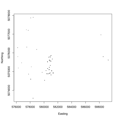
We can see the mapped trees in the same plots we mapped above. We've plotted each individual tree as a ., so all we can see at this scale is the cluster of dots that make up each plot.

Let's zoom in on a single plot:

plot(vst.loc$adjEasting[which(vst.loc$plotID=="WREF_085")], 
     vst.loc$adjNorthing[which(vst.loc$plotID=="WREF_085")], 
     pch=20, xlab="Easting", ylab="Northing")

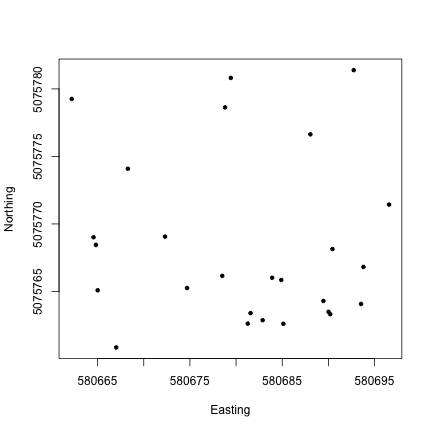
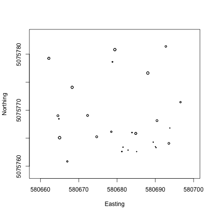
Now we can see the location of each tree within the sampling plot WREF_085. This is interesting, but it would be more interesting if we could see more information about each tree. How are species distributed across the plot, for instance?

We can plot the tree species at each location using the text() function and the vst.loc$taxonID field.

plot(vst.loc$adjEasting[which(vst.loc$plotID=="WREF_085")], 
     vst.loc$adjNorthing[which(vst.loc$plotID=="WREF_085")], 
     type="n", xlab="Easting", ylab="Northing")

text(vst.loc$adjEasting[which(vst.loc$plotID=="WREF_085")], 
     vst.loc$adjNorthing[which(vst.loc$plotID=="WREF_085")],
     labels=vst.loc$taxonID[which(vst.loc$plotID=="WREF_085")],
     cex=0.5)

Almost all of the mapped trees in this plot are either Pseudotsuga menziesii or Tsuga heterophylla (Douglas fir and Western hemlock), not too surprising at Wind River.

But suppose we want to map the diameter of each tree? This is a very common way to present a stem map, it gives a visual as if we were looking down on the plot from overhead and had cut off each tree at its measurement height.

Other than taxon, the attributes of the trees, such as diameter, height, growth form, and canopy position, are found in the vst_apparentindividual table, not in the vst_mappingandtagging table. We'll need to join the two tables to get the tree attributes together with their mapped locations.

The neonOS package contains the function joinTableNEON(), which can be used to do this. See the tutorial for the neonOS package for more details about this function.

veg <- joinTableNEON(vst.loc, 
                     vst$vst_apparentindividual,
                     name1="vst_mappingandtagging",
                     name2="vst_apparentindividual")

Now we can use the symbols() function to plot the diameter of each tree, at its spatial coordinates, to create a correctly scaled map of boles in the plot. Note that stemDiameter is in centimeters, while easting and northing UTMs are in meters, so we divide by 100 to scale correctly.

symbols(veg$adjEasting[which(veg$plotID=="WREF_085")], 
        veg$adjNorthing[which(veg$plotID=="WREF_085")], 
        circles=veg$stemDiameter[which(veg$plotID=="WREF_085")]/100/2, 
        inches=F, xlab="Easting", ylab="Northing")

If you are interested in taking the vegetation structure data a step further, and connecting measurements of trees on the ground to remotely sensed Lidar data, check out the Vegetation Structure and Canopy Height Model tutorial.

If you are interested in working with other terrestrial observational (TOS) data products, the basic techniques used here to find precise sampling locations and join data tables can be adapted to other TOS data products. Consult the Data Product User Guide for each data product to find details specific to that data product.

Locations for sensor data

Downloads of instrument system (IS) data include a file called sensor_positions.csv. The sensor positions file contains information about the coordinates of each sensor, relative to a reference location.

While the specifics vary, techniques are generalizable for working with sensor data and the sensor_positions.csv file. For this tutorial, let's look at the sensor locations for soil temperature (PAR; DP1.00041.001) at
the NEON Treehaven site (TREE) in July 2018. To reduce our file size, we'll use the 30 minute averaging interval. Our final product from this section is to create a depth profile of soil temperature in one soil plot.

If downloading data using the neonUtilties package is new to you, check out the neonUtilities tutorial.

This function will download about 7 MB of data as written so we have check.size =F for ease of running the code.

# load soil temperature data of interest 

soilT <- loadByProduct(dpID="DP1.00041.001", site="TREE",
                    startdate="2018-07", enddate="2018-07",
                    timeIndex=30, check.size=F)

## Attempting to stack soil sensor data. Note that due to the number of soil sensors at each site, data volume is very high for these data. Consider dividing data processing into chunks, using the nCores= parameter to parallelize stacking, and/or using a high-performance system.

Sensor positions file

Now we can specifically look at the sensor positions file.

# create object for sensor positions file

pos <- soilT$sensor_positions_00041



# view column names

names(pos)

##  [1] "siteID"                           "HOR.VER"                         
##  [3] "sensorLocationID"                 "sensorLocationDescription"       
##  [5] "positionStartDateTime"            "positionEndDateTime"             
##  [7] "referenceLocationID"              "referenceLocationIDDescription"  
##  [9] "referenceLocationIDStartDateTime" "referenceLocationIDEndDateTime"  
## [11] "xOffset"                          "yOffset"                         
## [13] "zOffset"                          "pitch"                           
## [15] "roll"                             "azimuth"                         
## [17] "locationReferenceLatitude"        "locationReferenceLongitude"      
## [19] "locationReferenceElevation"       "eastOffset"                      
## [21] "northOffset"                      "xAzimuth"                        
## [23] "yAzimuth"                         "publicationDate"

# view table

View(pos)

The sensor locations are indexed by the HOR.VER variable - see the file naming conventions page for more details.

Using unique() we can view all the location indices in this file.

unique(pos$HOR.VER)

##  [1] "001.501" "001.502" "001.503" "001.504" "001.505" "001.506" "001.507" "001.508" "001.509" "002.501"
## [11] "002.502" "002.503" "002.504" "002.505" "002.506" "002.507" "002.508" "002.509" "003.501" "003.502"
## [21] "003.503" "003.504" "003.505" "003.506" "003.507" "003.508" "003.509" "004.501" "004.502" "004.503"
## [31] "004.504" "004.505" "004.506" "004.507" "004.508" "004.509" "005.501" "005.502" "005.503" "005.504"
## [41] "005.505" "005.506" "005.507" "005.508" "005.509"

Soil temperature data are collected in 5 instrumented soil plots inside the tower footprint. We see this reflected in the data where HOR = 001 to 005. Within each plot, temperature is measured at 9 depths, seen in VER = 501 to 509. At some sites, the number of depths may differ slightly.

The x, y, and z offsets in the sensor positions file are the relative distance, in meters, to the reference latitude, longitude, and elevation in the file.

The HOR and VER indices in the sensor positions file correspond to the verticalPosition and horizontalPosition fields in soilT$ST_30_minute.

Note that there are two sets of position data for soil plot 001, and that one set has a positionEndDateTime date in the file. This indicates sensors either moved or were relocated; in this case there was a frost heave incident. You can read about it in the issue log, which is displayed on the Data Product Details page, and also included as a table in the data download:

soilT$issueLog_00041[grep("TREE soil plot 1", 
                     soilT$issueLog_00041$locationAffected),]

##      id parentIssueID            issueDate         resolvedDate       dateRangeStart         dateRangeEnd
## 1: 9328            NA 2019-05-23T00:00:00Z 2019-05-23T00:00:00Z 2018-11-07T00:00:00Z 2019-04-19T00:00:00Z
##                                                                                                                          locationAffected
## 1: D05 TREE soil plot 1 measurement levels 1-9 (HOR.VER: 001.501, 001.502, 001.503, 001.504, 001.505, 001.506, 001.507, 001.508, 001.509)
##                                                                                                                                                                                                                           issue
## 1: Soil temperature sensors were pushed or pulled out of the ground by 3 cm over winter, presumably due to freeze-thaw action. The exact timing of this is unknown, but it occurred sometime between 2018-11-07 and 2019-04-19.
##                                                                                        resolution
## 1: Sensor depths were updated in the database with a start date of 2018-11-07 for the new depths.

Since we're working with data from July 2018, and the change in sensor locations is dated Nov 2018, we'll use the original locations. There are a number of ways to drop the later locations from the table; here, we find the rows in which the positionEndDateTime field is empty, indicating no end date, and the rows corresponding to soil plot 001, and drop all the rows that meet both criteria.

pos <- pos[-intersect(grep("001.", pos$HOR.VER),
                      which(pos$positionEndDateTime=="")),]

Our goal is to plot a time series of temperature, stratified by depth, so let's start by joining the data file and sensor positions file, to bring the depth measurements into the same data frame with the data.

# paste horizontalPosition and verticalPosition together

# to match HOR.VER in the sensor positions file

soilT$ST_30_minute$HOR.VER <- paste(soilT$ST_30_minute$horizontalPosition,
                                    soilT$ST_30_minute$verticalPosition,
                                    sep=".")



# left join to keep all temperature records

soilTHV <- merge(soilT$ST_30_minute, pos, 
                 by="HOR.VER", all.x=T)

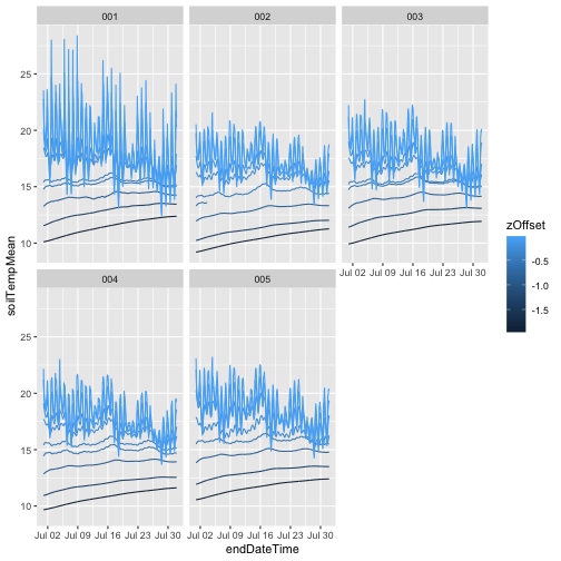
And now we can plot soil temperature over time for each depth. We'll use ggplot since it's well suited to this kind of stratification. Each soil plot is its own panel, and each depth is its own line:

gg <- ggplot(soilTHV, 
             aes(endDateTime, soilTempMean, 
                 group=zOffset, color=zOffset)) +
             geom_line() + 
        facet_wrap(~horizontalPosition)

gg

## Warning: Removed 1488 rows containing missing values (`geom_line()`).

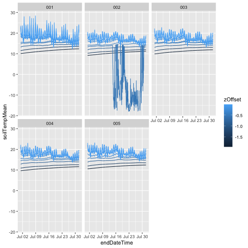
We can see that as soil depth increases, temperatures become much more stable, while the shallowest measurement has a clear diurnal cycle. We can also see that something has gone wrong with one of the sensors in plot 002. To remove those data, use only values where the final quality flag passed, i.e. finalQF = 0

gg <- ggplot(subset(soilTHV, finalQF==0), 
             aes(endDateTime, soilTempMean, 
                 group=zOffset, color=zOffset)) +
             geom_line() + 
        facet_wrap(~horizontalPosition)

gg