Workshop
NEON Data Institute 2017: Remote Sensing with Reproducible Workflows using Python
NEON
-
NEON Data Institutes provide critical skills and foundational knowledge for graduate students and early career scientists working with heterogeneous spatio-temporal data to address ecological questions.
Data Institute Overview
The 2017 Institute focuses on remote sensing of vegetation using open source tools and reproducible science workflows -- the primary programming language will be Python.
This Institute will be held at NEON headquarters in June 2017. In addition to the six days of in-person training, there are three weeks of pre-institute materials is to ensure that everyone comes to the Institute ready to work in a collaborative research environment. Pre-institute materials are online & individually paced, expect to spend 1-5 hrs/week depending on your familiarity with the topic.
Schedule
| Time | Day | Description |
|---|---|---|
| -- | Computer Setup Materials | |
| -- | 25 May - 1 June | Intro to NEON & Reproducible Science |
| -- | 2-8 June | Version Control & Collaborative Science with Git & GitHub |
| -- | 9-15 June | Documentation of Your Workflow with iPython/Jupyter Notebooks |
| -- | 19-24 June | Data Institute |
| 7:50am - 6:30 pm | Monday | Intro to NEON, Intro to HDF5 & Hyperspectral Remote Sensing |
| 8:00am - 6:30pm | Tuesday | Reproducible & Automated Workflows, Intro to LiDAR data |
| 8:00am - 6:30pm | Wednesday | Remote Sensing Uncertainty |
| 8:00am - 6:30pm | Thursday | Hyperspectral Data & Vegetation |
| 8:00am - 6:30pm | Friday | Individual/Group Applications |
| 9:00am - 1:00pm | Saturday | Group Application Presentations |
Key 2017 Dates
- Applications Open: 17 January 2017
- Application Deadline: 10 March 2017
- Notification of Acceptance: late March 2017
- Tuition payment due by: mid April 2017
- Pre-institute online activities: June 1-17, 2017
- Institute Dates: June 19-24, 2017
Instructors
Dr. Tristan Goulden, Associate Scientist-Airborne Platform, Battelle-NEON: Tristan is a remote sensing scientist with NEON specializing in LiDAR. He also co-lead NEON’s Remote Sensing IPT (integrated product team) which focusses on developing algorithms and associated documentation for all of NEON’s remote sensing data products. His past research focus has been on characterizing uncertainty in LiDAR observations/processing and propagating the uncertainty into downstream data products. During his PhD, he focused on developing uncertainty models for topographic attributes (elevation, slope, aspect), hydrological products such as watershed boundaries, stream networks, as well as stream flow and erosion at the watershed scale. His past experience in LiDAR has included all aspects of the LIDAR workflow including; mission planning, airborne operations, processing of raw data, and development of higher level data products. During his graduate research he applied these skills on LiDAR flights over several case study watersheds of study as well as some amazing LiDAR flights over the Canadian Rockies for monitoring change of alpine glaciers. His software experience for LiDAR processing includes Applanix’s POSPac MMS, Optech’s LMS software, Riegl’s LMS software, LAStools, Pulsetools, TerraScan, QT Modeler, ArcGIS, QGIS, Surfer, and self-written scripts in Matlab for point-cloud, raster, and waveform processing.
Bridget Hass, Remote Sensing Data Processing Technician, Battelle-NEON: Bridget’s daily work includes processing LiDAR and hyperspectral data collected by NEON's Aerial Observation Platform (AOP). Prior to joining NEON, Bridget worked in marine geophysics as a shipboard technician and research assistant. She is excited to be a part of producing NEON's AOP data and to share techniques for working with this data during the 2017 Data Institute.
Dr. Naupaka Zimmerman, Assistant Professor of Biology, University of San Francisco: Naupaka’s research focuses on the microbial ecology of plant-fungal interactions. Naupaka brings to the course experience and enthusiasm for reproducible workflows developed after discovering how challenging it is to keep track of complex analyses in his own dissertation and postdoctoral work. As a co-founder of the International Network of Next-Generation Ecologists and an instructor and lesson maintainer for Software Carpentry and Data Carpentry, Naupaka is very interested in providing and improving training experiences in open science and reproducible research methods.
Dr. Paul Gader, Professor, University of Florida:
Paul is a Professor of Computer & Information Science & Engineering (CISE)
at the Engineering School of Sustainable Infrastructure and the Environment
(ESSIE) at the University of Florida(UF). Paul received his Ph.D. in Mathematics
for parallel image processing and applied mathematics research in 1986 from UF,
spent 5 years in industry, and has been teaching at various universities since 1991.
His first research in image processing was in 1984 focused on algorithms
for detection of bridges in Forward Looking Infra-Red (FLIR) imagery. He has
investigated algorithms for land mine research since 1996, leading a team that
produced new algorithms and real-time software for a sensor system currently
operational in Afghanistan. His landmine detection projects involve algorithm
development for data generated from hand-held, vehicle-based, and airborne
sensors, including ground penetrating radar, acoustic/seismic, broadband IR
(emissive and reflective bands), emissive and reflective hyperspectral imagery,
and wide-band electro-magnetic sensors. In the past few years, he focused on
algorithms for imaging spectroscopy. He is currently researching nonlinear
unmixing for object and material detection, classification and segmentation, and
estimating plant traits. He has given tutorials on nonlinear unmixing at
International Conferences. He is a Fellow of the Institute of Electrical and
Electronic Engineers, an Endowed Professor at the University of Florida, was
selected for a 3-year term as a UF Research Foundation Professor, and has over
100 refereed journal articles and over 300 conference articles.
This page includes all of the materials needed for the Data Institute including the pre-institute materials. Please use the sidebar menu to find the appropriate week or day. If you have problems with any of the materials please email us or use the comments section at the bottom of the appropriate page.
Pre-Institute: Computer Set Up Materials
It is important that you have your computer setup, prior to diving into the pre-institute materials in week 2! Please review the links below to setup the laptop you will be bringing to the Data Institute.
Let's Get Your Computer Setup!
Go to each of the following tutorials and complete the directions to set your computer up for the Data Institute.
Install Git, Bash Shell, Python
Set up GitHub Working Directory - Quick Intro to Bash
Install QGIS & HDFView
Pre-Institute Week 1: NEON & Reproducible Science
In the first week of the pre-institute activities, we will review the NEON project. We will also provide you with a general overview of reproducible science. Over the next few weeks will we ask you to review materials and submit something that demonstrates you have mastered the materials.
Learning Objectives
After completing these activities, you will be able to:
- Describe the NEON project, the data collected, and where to access more information about the project.
- Know how to access other code resources for working with NEON data.
- Explain why reproducible workflows are useful and important in your research.
Week 1 Assignment
After reviewing the materials below, please write up a summary of a project that you are interested working on at the Data Institute. Be sure to consider what data you will need (NEON or other). You will have time to refine your idea over the next few weeks. Save this document as you will submit it next week as a part of week 2 materials!
Deadline: Please complete this by Thursday June 1st @ 11:59 MDT.
Week 1 Materials
Please carefully read and review the materials below:
Introduction to the National Ecological Observatory Network (NEON)
The Importance of Reproducible Science
"Reproducibility is a key tenet of the scientific process that dictates the reliability and generality of results and methods." From Powers, S. M., and S. E. Hampton (2019), Open science, reproducibility, and transparency in ecology (Abstract)
This lesson introduces the core principles of reproducible science in ecology and provides practical ways to apply them in your own research workflows.
In ecological science, reproducibility is especially important because observations are often context-dependent in space and time, so transparent and computationally reproducible workflows are critical for credible science, management, and policy decisions.
NEON data are especially well suited for reproducible ecological workflows because they are collected using standardized protocols across sites and time, include rich metadata and documentation, and are delivered in formats that make analyses easier to trace, rerun, and compare.
Learning Objectives
At the end of this activity, you will be able to:
- Summarize the four facets of reproducibility.
- Describe several ways that reproducible workflows can improve your workflow and research.
- Explain several ways you can incorporate reproducible science techniques into your own research.
Getting Started with Reproducible Science
This lesson summarizes key concepts about reproducible science, adapted from the Reproducible Science Curriculum.
Why use reproducible methods?
Reproducible methods make science more efficient, more collaborative, and more trustworthy across the full lifecycle of a project. Some benefits to reproducibility include:
- More efficient, less redundant.
- Allows for continuity in your own work over time.
- Facilitates collaboration, review, and re-use by others.
- Provides stronger transparency and trust in results.
What research products should be shareable?
To support reproducibility, key research products should be publicly available in forms that others can find and understand:
- Data
- Code
- Documentation about methods and workflow
Who needs to understand your workflow?
- Collaborators
- Peer reviewers and journal editors
- The broader scientific community
- The public
The Four Facets of Reproducibility
Reproducibility is often discussed as one idea, but in practice it has several connected facets. Improving all four helps make your work more robust and more useful to others.
- Organization: use clear file structures, informative file names, and explicit separation of raw, intermediate, and final outputs.
- Automation: prefer scripts over point-and-click steps so analyses can be rerun, modified, and reviewed efficiently.
- Documentation: record decisions, code purpose, inputs/outputs, and workflow steps so others (and your future self) can understand the work.
- Dissemination: share data, code, and workflows in accessible repositories and formats so others can find, evaluate, and build on your results.
In practice: You can be strong in one facet and weak in another, so reproducibility is usually a work in progress rather than an all-or-nothing goal. For example, sharing code without data provenance may limit reproducibility even when the analysis itself is well documented.
How Reproducible Workflows Improve Research
Reproducible workflows provide benefits both during a project and after publication.
- Fewer errors and faster debugging: scripted workflows make mistakes easier to detect and fix.
- Easier collaboration: shared conventions (file naming, documentation, version control) reduce friction across teams.
- More efficient updates: when data are revised, automated workflows can rebuild results quickly.
- Greater trust and re-use: transparent methods improve confidence and make it easier for others to build on your work.
- Stronger scientific impact: reproducible outputs are more likely to be re-analyzed, cited, and used for synthesis.
Incorporating Reproducible Science Into Your Workflow
You do not need to adopt everything at once. Start with small, high-impact changes and build over time.
Quick Wins (start this week)
- Use descriptive file names and a consistent folder structure.
- Keep raw data read-only; write processed outputs to separate directories.
- Record software versions and package dependencies.
- Add a project
READMEwith goals, inputs, and run instructions.
Next Steps (this month)
- Move repeated analyses from point-and-click tools into scripts.
- Use version control (for example, Git) for code and documentation.
- Add lightweight quality checks for expected rows, columns, units, and ranges.
- Archive analysis-ready data and scripts with a persistent identifier (DOI).
Advanced Practices (ongoing)
- Build end-to-end pipelines that regenerate figures and tables.
- Use computational environments (for example, containers) to improve run-to-run consistency.
- Add executable reports/notebooks that pair narrative, code, and outputs.
- Include clear licensing, citation, and contribution guidance for re-use.
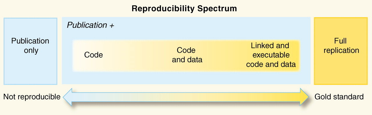
Practical Challenges and Tradeoffs
Adopting reproducible methods often requires more setup time at the beginning. However, this up-front investment usually saves time later by making analyses easier to update, repeat, and explain. Moving towards reproducibility can be approached with a "good-better-best" framework. See the figure below to assess where your work lies on the reproducability spectrum.
How reproducible is your current research?
View Reproducible Science Checklist
Thought Questions: Have a look at the reproducible science check list linked above and answer the following questions:
- Do you currently apply any of the items in the checklist to your research?
- Are there elements in the list that you are interested in incorporating into your workflow? If so, which ones?
Self-Check Quiz
Use this quick quiz to check your understanding of the learning objectives.
-
Which list matches the four facets from the NEON reproducible science slides?
A. Computation, Statistics, Visualization, Reporting B. Organization, Automation, Documentation, Dissemination C. Planning, Coding, Publishing, Archiving D. Collection, Cleaning, Modeling, Interpretation
-
Which practice is most aligned with the Organization facet?
A. Using informative file names and a clear directory structure B. Writing results directly over raw input data C. Keeping steps undocumented but fast D. Sharing only a figure in a slide deck
-
Why is scripting preferred over manual steps for many analyses?
A. It always requires less up-front time B. It makes methods harder for collaborators to inspect C. It supports efficient reruns and updates over time D. It removes the need for version control
-
Which audiences may need access to your research workflow?
A. Principal investigators B. Peer reviewers C. Collaborators, peer reviewers/editors, the scientific community, and the public D. Data managers
-
Which option best reflects the Dissemination facet?
A. Publishing ends the workflow; no further sharing is needed B. Share data snapshots and workflows in accessible platforms (for example, repositories and notebook-sharing tools) C. Keep data private unless requested by email D. Share code only if journal reviewers ask for it
Quiz Key
- B
- A
- C
- C
- B
Reflection Prompts
Use these prompts for discussion, journaling, or a short assignment.
- Which of the four facets is currently strongest in your workflow? Which is weakest?
- Identify one analysis step in your current project that is hard to rerun. What single change would make it easier to reproduce?
- If a collaborator joined your project tomorrow, what three artifacts (files, notes, metadata, or scripts) would help them reproduce your results fastest?
- What is one reproducibility practice you can adopt this week and one you can adopt this month?
- How might improved transparency change trust in your results for a policy, management, or stakeholder audience?
Additional Readings and Resources (optional)
Resources
- Nature magazine's special archive on the Challenges of Irreproducible Science.
- Open-access issue of Ecography focusing on reproducible ecology and software practices.
- Hampton, S. E., et al. (2015). Open science, reproducibility, and transparency in ecology. Ecological Applications.
- NASA Open Science (TOPS): Open Science at NASA.
- The Turing Way (living handbook): The Turing Way: A handbook for reproducible, ethical, and collaborative data science.
Hands-on tutorials and workshops
- NASA Open Science training catalog (includes Open Science 101 and Open Science Essentials): Open Science Training.
- Software Carpentry lesson (R): R for Reproducible Scientific Analysis.
- Reproducible Data Science in Python: Textbook on reproducible workflows in Python.
Pre-Institute Week 2: Version Control & Collaborative Science
The goal of the pre-institute materials is to ensure that everyone comes to the Institute ready to work in a collaborative research environment. If you recall, from last week, the four facets of reproducibility are documentation, organization, automation, and dissemination.
This week we will focus on learning to use tools to help us with these facets: Git and GitHub. The Git Hub environment supports both a collaborative approach to science through code sharing and dissemination, and a powerful version control system that supports both efficient project organization, and an effective way to save your work.
Learning Objectives
After completing these activities, you will be able to:
- Summarize the key components of a version control system
- Know how to setup a GitHub account
- Know how to setup Git locally
- Work in a collaborative workflow on GitHub
Week 2 Assignment
The assignment for this week is to revise the Data Institute capstone project summary that you developed last week. You will submit your project summary, with a brief biography to introduce yourself, to a shared GitHub repository.
Please complete this assignment by Thursday June 8th @ 11:59 PM MDT.
If you are familiar with forked repos and pull requests GitHub, and the use of Git in the command line, you may be able to complete the assignment without viewing the
tutorials.
Assignment: Version Control with GitHub
Week 2 Materials
Please complete each of the short tutorials in this series.
Version Control with GitHub
Pre-Institute Week 3: Documentation of Your Workflow
In week 3, you will use Jupyter Notebooks (formerly iPython Notebooks) to document code and efficiently publish code results & outputs. You will practice your Git skills by publishing your work in the NEON-WorkWithData/DI-NEON-participants GitHub repository.
In addition, you will watch a video that provides an overview of the NEON Vegitation Indices that are available as data products in preparation for Monday's materials.
Learning Objectives
After completing these activities, you will be able to:
- Use Jupyter Notebooks to create code with formatted context text
- Describe the value of documented workflows
Week 3 Assignment, Part 1
Please complete the activity and submit your work to the GitHub repo by Thursday June 17th at 11:59 MDT.
If you are familiar with using Jupyter Notebooks to document your workflow and knitting to HTML then you may be able to complete the assignment without viewing the tutorials.
Assignment: Reproducible Workflows with Jupyter Notebooks
In this tutorial you will learn how to open a .tiff file in Jupyter Notebook and learn about kernels.
The goal of the activity is simply to ensure that you have basic
familiarity with Jupyter Notebooks and that the environment, especially the
gdal package is correctly set up before you pursue more programming tutorials. If you already
are familiar with Jupyter Notebooks using Python, you may be able to complete the
assignment without working through the instructions.
This will be accomplished by: *Create a new Jupyter kernel *Download a GEOTIFF file *Import file onto Jupyter Notebooks *Check the raster size
Assignment: Open a Tiff File in Jupyter Notebook
Set up Environment
First, we will set up the environment as you would need for each of the live coding sections of the Data Institute. The following directions are copied over from the Data Institute Set up Materials.
In your terminal application, navigate to the directory (cd) that where you
want the Jupyter Notebooks to be saved (or where they already exist).
We need to create a new Jupyter kernel for the Python 3.8 conda environment (py38) that Jupyter Notebooks will use.
In your Command Prompt/Terminal, type:
python -m ipykernel install --user --name py34 --display-name "Python 3.8 NEON-RSDI"
In your Command Prompt/Terminal, navigate to the directory (cd) that you
created last week in the GitHub materials. This is where the Jupyter Notebook
will be saved and the easiest way to access existing notebooks.
###Open Jupyter Notebook Open Jupyter Notebook by typing into a command terminal:
jupyter notebook
Once the notebook is open, check which version of Python you are in.
 # Check what version of Python.  Should be 3.8.
 import sys
 sys.version
To ensure that the correct kernel will operate, navigate to Kernel in the menu, select Kernel/Restart Kernel And Clear All Outputs.

You should now be able to work in the notebook.
#Download the digital terrain model (GEOTIFF file) Download the NEON GeoTiFF file of a digital terrain model (dtm) of the San Joaquin Experimental Range. Click this link to download dtm data: https://ndownloader.figshare.com/articles/2009586/versions/10. This will download a zippped full of data originally from a NEON data carpentry tutorial (https://datacarpentry.org/geospatial-workshop/data/).
Once downloaded, navigate through the folder to C:NEON-DS-Airborne-Remote-Sensing.zip\NEON-DS-Airborne-Remote-Sensing\SJER\DTM and save this file onto your own personal working directory. .
###Open GEOTIFF file in Jupyter Notebooks using gdal
The gdal package that occasionally has problems with some versions of Python.
Therefore test out loading it using:
import gdal.
If you have trouble, ensure that 'gdal' is installed on your current environment.
Establish your directory
Place the downloaded dtm file in a repository of your choice (or your current working directory). Navigate to that directory. wd= '/your-file-path-here' #Input the directory to where you saved the .tif file
Import the TIFF
Import the NEON GeoTiFF file of the digital terrain model (DTM)
from San Joaquin Experimental Range. Open the file using the gdal.Open command.Determine the size of the raster and (optional) plot the raster.
#Use GDAL to open GEOTIFF file stored in your directory SJER_DTM = gdal.Open(wd + 'SJER_dtmCrop.tif')>
#Determine the raster size.
SJER_DTM.RasterXSize
Add in both code chunks and text (markdown) chunks to fully explain what is done. If you would like to also plot the file, feel free to do so.
Push .ipynb to GitHub.
When finished, save as a .ipynb file.
Week 3 Materials
Please complete each of the short tutorials in this series.
Document Your Code with Jupyter Notebooks
Week 3 Assignment, Part 2
On the first day of the course, we will be working with hyperspectral data. Various indices, including the Normalized Difference Vegetation Index (NDVI), are common data products from hyperspectral data. In preparation for this content, please watch this video of David Hulslander discussing NEON remote sensing vegetation indices & data products.
Monday: HDF5, & Hyperspectral Data
Learning Objectives
After completing these activities, you will be able to:
- Open and work with raster data stored in HDF5 format in Python
- Explain the key components of the HDF5 data structure (groups, datasets and attributes)
- Open and use attribute data (metadata) from an HDF5 file in Python
Morning: Intro to NEON & HDF5
All activities are held in the the Classroom unless otherwise noted.
| Time | Topic | Instructor/Location |
|---|---|---|
| 8:00 | Welcome & Introductions | |
| 8:30 | Introduction to the National Ecological Observatory Network | Megan Jones |
| 9:00 | Introduction to NEON AOP (download presentation) | Nathan Leisso |
| 9:30 | NEON RGB Imagery (download presentation) | Bill Gallery |
| 10:00 | Introduction to the HDF5 File Format (download PDF) | Ted Haberman |
| 10:30 | BREAK | |
| 10:45 | NEON Tour | |
| 12:00 | LUNCH | Classroom/Patio |
Afternoon: Hyperspectral Remote Sensing
| Time | Topic | Instructor/Location |
|---|---|---|
| 13:00 | An Introduction to Hyperspectral Remote Sensing (related video) | Tristan Goulden |
| 13:20 | Work with Hyperspectral Remote Sensing data & HDF5 | |
| Explore NEON HDF5 format with Viewer | Tristan | |
| NEON AOP Hyperspectral Data in HDF5 format with Python | Bridget Hass | |
| Band Stacking, RGB & False Color Images, and Interactive Widgets in Python | Bridget | |
| 15:00 | BREAK | |
| Plot Spectral Signatures | Bridget | |
| Calculate NDVI | Bridget | |
| Calculate Other Indices; Small Group Coding | Megan | |
| 17:30 | GitHub Workflow | Naupaka Zimmerman |
| 18:00 | End of Day Wrap Up | Megan |
Additional Information
This morning, we will be touring the NEON facilities including several labs. Please wear long pants and close-toed shoes to conform to lab safety standards. Many individuals find the temperature of the classroom where the Data Institute is held to be cooler than they prefer. We recommend you bring a sweater or light jacket with you. You will have the opportunity to eat your lunch on an outdoor patio - hats, sunscreen, and sunglasses may be appreciated.
Additional Resources
Participants looking for more background on the HDF5 format may find these tutorials useful.
- Hierarchical Data Formats - What is HDF5? tutorial
- Explore HDF5 Files using the HDF5View Tool tutorial
During the 2016 Data Institute, Dr. Dave Schimel gave a presentation on the importance of "Big Data, Open Data, and Biodiversity" and is very much related to the themes of this Data Institute. If interested you can watch the video here.
Tuesday: Lidar Data & Reproducible Workflows
In the morning, we will focus on data workflows, organization and automation as a means to write more efficient, usable code. Later, we will review the basics of discrete return and full waveform lidar data. We will then work with some NEON lidar derived raster data products.
Learning Objectives
After completing these activities, you will be able to:
- Explain the difference between active and passive sensors.
- Explain the difference between discrete return and full waveform LiDAR.
- Describe applications of LiDAR remote sensing data in the natural sciences.
- Describe several NEON LiDAR remote sensing data products.
- Explain why modularization is important and supports efficient coding practices.
- How to modularize code using functions.
- Integrate basic automation into your existing data workflow.
Morning: Reproducible Workflows
| Time | Topic | Instructor/Location |
|---|---|---|
| 8:00 | Automate & Modularize Workflows | Naupaka Zimmerman |
| 10:30 | BREAK | |
| 10:45 | Automate & Modularize Workflows, cont. | |
| 12:00 | LUNCH | Classroom/Patio |
Afternoon: Lidar
| Time | Topic | Instructor/Location |
|---|---|---|
| 13:00 | An Introduction to Discrete Lidar (video) | Tristan Goulden |
| An Introduction to Waveform Lidar (related video) | Keith Krause | |
| OpenTopography as a Data Source (download PDF) | Benjamin Gross | |
| 14:00 | Rasters & TIFF tags | Tristan |
| 14:15 | Classify a Raster using Threshold Values | Bridget |
| Mask a Raster using Threshold Values | Bridget | |
| Create a Hillshade from a Terrain Raster in Python | Bridget | |
| 15:00 | BREAK | |
| 15:15 | Lidar Small Group Coding Activity | Tristan & Bridget |
| 18:00 | End of Day Wrap Up | Megan Jones |
Wednesday: Uncertainty
Today, we will focus on the importance of uncertainty when using remote sensing data.
Learning Objectives
After completing these activities, you will be able to:
- Measure the differences between a metric derived from remote sensing data and the same metric derived from data collected on the ground.
| Time | Topic | Instructor/Location |
|---|---|---|
| 8:00 | Uncertainty & Lidar Data Presentation (video) | Tristan Gouldan |
| 8:40 | Exploring Uncertainty in LiDAR Data | Tristan |
| 10:30 | BREAK | |
| 10:45 | Lidar Uncertainty cont. | Tristan |
| 12:00 | LUNCH | Classroom/Patio |
| 13:00 | Spectral Calibration & Uncertainty Presentation (video) | Nathan Leisso |
| 13:30 | Hyperspectral Variation Uncertainty Analysis in Python | Tristan |
| Assessing Spectrometer Accuracy using Validation Tarps with Python | Tristan | |
| 15:00 | BREAK | |
| 15:50 | Uncertainty in BRDF Flight Data Products at Three Locations presentation | Amanda Roberts |
| Hyperspectral Validation, cont. | Tristan | |
| 18:00 | End of Day Wrap Up | Megan Jones |
Thursday: Applications
On Thursday, we will begin to think about the different types of analysis that we can do by fusing LiDAR and hyperspectral data products.
Learning Objectives
After completing these activities, you will be able to:
- Classify different spectra from a hyperspectral data product
- Map the crown of trees from hyperspectral & lidar data
- Calculate biomass of vegetation
| Time | Topic | Instructor/Location |
|---|---|---|
| 8:00 | Applications of Remote Sensing | Paul Gader |
| 9:00 | NEON Vegetation Data (related video, download PDF ) | Katie Jones |
| NEON Foliar Chemistry & Soil Chemistry Data and Microbial Data (video) | Samantha Weintraub | |
| 9:40 | Classification of Spectra | Paul |
| Classification of Hyperspectral Data with Ordinary Least Squares in Python, (download PDF ) | Paul | |
| Classification of Hyperspectral Data with Principal Components Analysis in Python, (download PDF ) | Paul | |
| Classification of Hyperspectral Data with SciKit & SVM in Python, (download PDF ) | Paul | |
| 10:30 | BREAK | |
| 10:45 | Classification of Spectra, cont. | Paul |
| 12:00 | LUNCH | Classroom/Patio |
| 13:00 | Tree Crown Mapping | Paul |
| 15:00 | BREAK | |
| 15:15 | Biomass Calculations | Tristan Goulden |
| 17:30 | Capstone Brainstorm & Group Selection | Megan Jones |
Calculate Vegetation Biomass from LiDAR Data in Python
In this tutorial, we will calculate the biomass for a section of the SJER site. We will be using the Ecosystem structure, or Canopy Height Model (CHM), derived from discrete lidar, as well as training data derived from NEON Vegetation structure data. This tutorial will calculate Biomass for individual trees in the forest.
Learning Objectives
After completing this tutorial, you will be able to:
- Learn how to apply a guassian smoothing kernel for high-frequency spatial filtering
- Apply a watershed segmentation algorithm for delineating tree crowns
- Calculate biomass predictor variables from a CHM
- Setup training data for Biomass predictions
- Apply a Random Forest machine learning approach to calculate biomass
Things You’ll Need To Complete This Tutorial
To complete this tutorial, you will need:
- Python version 3.9 or higher
- Create a NEON user account
- Generate an API token for downloading data
Install Python Packages
- gdal
- scipy
- scikit-learn
- scikit-image
- neonutilities
- python-dotenv
The following packages should be part of the standard conda installation:
- os
- sys
- numpy
- matplotlib
Download Data
The Canopy Height Model data will be downloaded programmatically at the start of the script. Download the training data by clicking on the link below.
Download the Training Data: SJER_Biomass_Training.csv and save it in your working directory.
In this tutorial, we will calculate the biomass for a section of the SJER site. We will be using the Canopy Height Model discrete LiDAR data product as well as NEON field data on vegetation data. This tutorial will calculate biomass for individual trees in the forest.
Calculating biomass using this method consists of four primary steps:
- Delineate individual tree crowns using watershed segmentation
- Calculate predictor variables for all individual trees
- Collect training data
- Apply a Random Forest regression model to estimate biomass from the predictor variables
In this tutorial we use a Random Forest (RF) machine learning algorithm for relating the predictor variables to biomass (part 4). The predictor variables were selected following suggestions by Gleason et al. (2012) and biomass estimates were determined from the stem diameter measurements (diameter at breast height, or DBH) from NEON's vegetation structure data product, following relationships given in Jenkins et al. (2003).
Get Started
First, import the Python packages required to run various parts of the script:
import os, sys, dotenv
from osgeo import gdal, osr
import matplotlib.pyplot as plt
import neonutilities as nu
import numpy as np
import pandas as pd
import rasterio as rio
from rasterio.plot import show, show_hist
from scipy import ndimage as ndi
Next, we will add libraries from scikit-learn which will help with the watershed delination, determination of predictor variables and random forest algorithm
#Import biomass specific libraries
from skimage.segmentation import watershed
from skimage.feature import peak_local_max
from skimage.measure import regionprops
from sklearn.ensemble import RandomForestRegressor
We also need to specify the directory where we will find and save the data needed for this tutorial. You may need to change this line to follow a different working directory structure, or to suit your local machine. I have decided to save my data in the following directory:
data_path = "C:\data"
Define functions
Now we will define a few functions that allow us to pull metrics from the CHM data and get predictor variables.
-
crown_geometric_volume_pct: function to get the tree height and crown volume percentiles
def crown_geometric_volume_pct(tree_data,min_tree_height,pct):
    p = np.percentile(tree_data, pct)
    tree_data_pct = [v if v < p else p for v in tree_data]
    crown_geometric_volume_pct = np.sum(tree_data_pct - min_tree_height)
    return crown_geometric_volume_pct, p
-
get_predictors: function to get the predictor variables from the CHM data
def get_predictors(tree,chm_array, labels):
    indexes_of_tree = np.asarray(np.where(labels==tree.label)).T
    tree_crown_heights = chm_array[indexes_of_tree[:,0],indexes_of_tree[:,1]]

    full_crown = np.sum(tree_crown_heights - np.min(tree_crown_heights))

    crown50, p50 = crown_geometric_volume_pct(tree_crown_heights,tree.min_intensity,50)
    crown60, p60 = crown_geometric_volume_pct(tree_crown_heights,tree.min_intensity,60)
    crown70, p70 = crown_geometric_volume_pct(tree_crown_heights,tree.min_intensity,70)

    return [tree.label,
            float(tree.area),
            tree.major_axis_length,
            tree.max_intensity,
            tree.min_intensity,
            p50, p60, p70,
            full_crown,
            crown50, crown60, crown70]
-
output_raster: function to write out intermediate rasters and the final biomass raster
def output_raster(output_path, array, profile, dtype="float32", nodata=None):
    out_profile = profile.copy()
    out_profile.update(driver="GTiff", count=1, dtype=dtype, nodata=nodata)

    with rio.open(output_path, "w", **out_profile) as dst:
        dst.write(np.asarray(array, dtype=dtype), 1)
Download CHM Data
As of June 2026, NEON requires an API token for data downloads, to reduce bot scraping and improve user support. Tokens can be generated in NEON data portal user accounts - log in to your account or create one, and go to the API Tokens section. For best practices in storing and using tokens, follow the instructions here. Once you've set up your token as an environment variable, you can load it using the python-dotenv package as follows, optionally specifying the path to the .env file in load_dotenv().
dotenv.load_dotenv()
token = os.environ.get("NEON_TOKEN")
# download the CHM data to the C:/data directory - change this if desired
nu.by_tile_aop(dpid='DP3.30015.001',
               site='SJER',
               year=2018,
               easting=256000,
               northing=4106000,
               token=token,
               savepath=r'C:\data')
Provisional NEON data are not included. To download provisional data, use input parameter include_provisional=True.


Continuing will download 2 NEON data files totaling approximately 551.9 KB. Do you want to proceed? (y/n)  y


Downloading 2 NEON data files totaling approximately 551.9 KB

100%|█████████████████████████████████████████████████████████████████████████████████████████████████████████████████████████| 2/2 [00:00<00:00,  2.64it/s]
chm_dir = os.path.expanduser(r"C:\data\DP3.30015.001\neon-aop-products\2018")

for root, dirs, files in os.walk(chm_dir):
    for file in files:
        if file.endswith('.tif'):
            chm_file = os.path.join(root, file)
            print(chm_file)
C:\data\DP3.30015.001\neon-aop-products\2018\FullSite\D17\2018_SJER_3\L3\DiscreteLidar\CanopyHeightModelGtif\NEON_D17_SJER_DP3_256000_4106000_CHM.tif
Plot CHM Data
With everything set up, we can now start working with our data by define the file path to our CHM file. Note that you will need to change this and subsequent filepaths according to your local machine.
When we output the results, we will want to include the same file information as the input, so we will gather the file name information.
Now we will read in the CHM data using rasterio ...
chm_dataset = rio.open(chm_file)
..., and plot it.
show(chm_dataset);
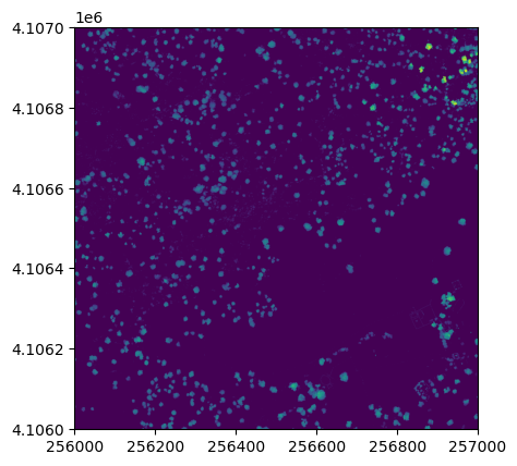
It looks like SJER primarily has low vegetation with scattered taller trees.
Read in the CHM as an array, as well as other relevant info we'll use later on:
with rio.open(chm_file) as src:
    # Read CHM values and keep ground/no-data as 0 for downstream segmentation steps
    chm_array = src.read(1, masked=True).filled(0).astype(np.float32)
    chm_profile = src.profile.copy()
    chm_bounds = src.bounds
    extent = (chm_bounds.left, chm_bounds.right, chm_bounds.bottom, chm_bounds.top)
    chm_name = os.path.basename(chm_file)
Create Filtered CHM
Now we will use a Gaussian smoothing kernal (convolution) across the data set to remove spurious high vegetation points. This will help ensure we are finding the treetops properly before running the watershed segmentation algorithm.
For different forest types it may be necessary to change the input parameters. Information on the function can be found in the SciPy documentation.
Of most importance are the second and fifth inputs. The second input defines the standard deviation of the Gaussian smoothing kernal. Too large a value will apply too much smoothing, too small and some spurious high points may be left behind. The fifth, the truncate value, controls after how many standard deviations the Gaussian kernal will get cut off (since it theoretically goes to infinity).
#Smooth the CHM using a gaussian filter to remove spurious points
chm_array_smooth = ndi.gaussian_filter(chm_array,2,mode='constant',cval=0,truncate=2.0)
chm_array_smooth[chm_array==0] = 0
Now save a copy of filtered CHM. We will later use this in our code, so we'll output it into our data directory.
# Save the smoothed CHM using rasterio
output_raster(
    os.path.join(data_path, 'chm_filter.tif'),
    chm_array_smooth,
    chm_profile,
    dtype="float32",
    nodata=0
    )
Determine local maximums
Now we will run an algorithm to determine local maximums within the image. Setting indices to False returns a raster of the maximum points, as opposed to a list of coordinates. The footprint parameter is an area where only a single peak can be found. This should be approximately the size of the smallest tree. Information on more sophisticated methods to define the window can be found in Chen (2006).
# Calculate local maximum points for filtered and unfiltered CHM
footprint = np.ones((5, 5), dtype=bool)

# Unfiltered maxima
local_max_coords_unfiltered = peak_local_max(
    chm_array,
    footprint=footprint,
    exclude_border=False
    )
local_maxi_unfiltered = np.zeros_like(chm_array, dtype=bool)
if local_max_coords_unfiltered.size > 0:
    local_maxi_unfiltered[tuple(local_max_coords_unfiltered.T)] = True

# Filtered maxima (used downstream for segmentation)
local_max_coords = peak_local_max(
    chm_array_smooth,
    footprint=footprint,
    exclude_border=False
    )
local_maxi = np.zeros_like(chm_array_smooth, dtype=bool)
if local_max_coords.size > 0:
    local_maxi[tuple(local_max_coords.T)] = True
Our new object local_maxi is an array of boolean values where each pixel is identified as either being the local maximum (True) or not being the local maximum (False).
local_maxi
array([[False, False, False, ..., False, False, False],
       [False, False,  True, ..., False, False, False],
       [False, False, False, ..., False, False, False],
       ...,
       [False, False, False, ..., False, False, False],
       [False, False, False, ..., False, False, False],
       [False, False, False, ..., False, False, False]],
      shape=(1000, 1000))
This is helpful, but it can be difficult to visualize boolean values. We can convert this boolean array to an numeric format to use this function. Booleans convert easily to integers with values of False=0 and True=1 using the .astype(int) method.
local_maxi.astype(int)
array([[0, 0, 0, ..., 0, 0, 0],
       [0, 0, 1, ..., 0, 0, 0],
       [0, 0, 0, ..., 0, 0, 0],
       ...,
       [0, 0, 0, ..., 0, 0, 0],
       [0, 0, 0, ..., 0, 0, 0],
       [0, 0, 0, ..., 0, 0, 0]], shape=(1000, 1000))
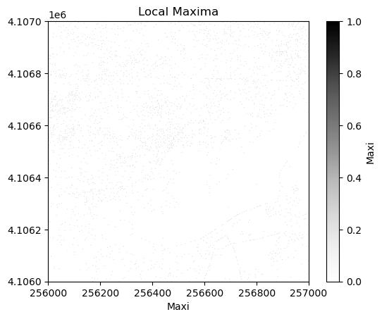
Next we can plot the raster of local maximums by coercing the boolean array into an array of integers inline. The following figure shows the difference in finding local maximums for a filtered vs. non-filtered CHM.
We will save the graphics (.png) in an outputs folder sister to our working directory and data outputs (.tif) to our data directory.
# Plot the local maximums
plt.figure(2)
plt.imshow(local_maxi.astype(int), cmap='Greys', extent=extent, origin='upper', vmin=0, vmax=1)
plt.title('Local Maxima')
plt.xlabel('Maxi')
plt.colorbar(label='Maxi')

plt.savefig(data_path+chm_name[0:-4]+ '_Maximums.png',
            dpi=300,orientation='landscape',
            bbox_inches='tight',pad_inches=0.1)

output_raster(
    os.path.join(data_path, 'maximum.tif'),
    local_maxi.astype(np.uint8),
    chm_profile,
    dtype="uint8",
    nodata=0
    )
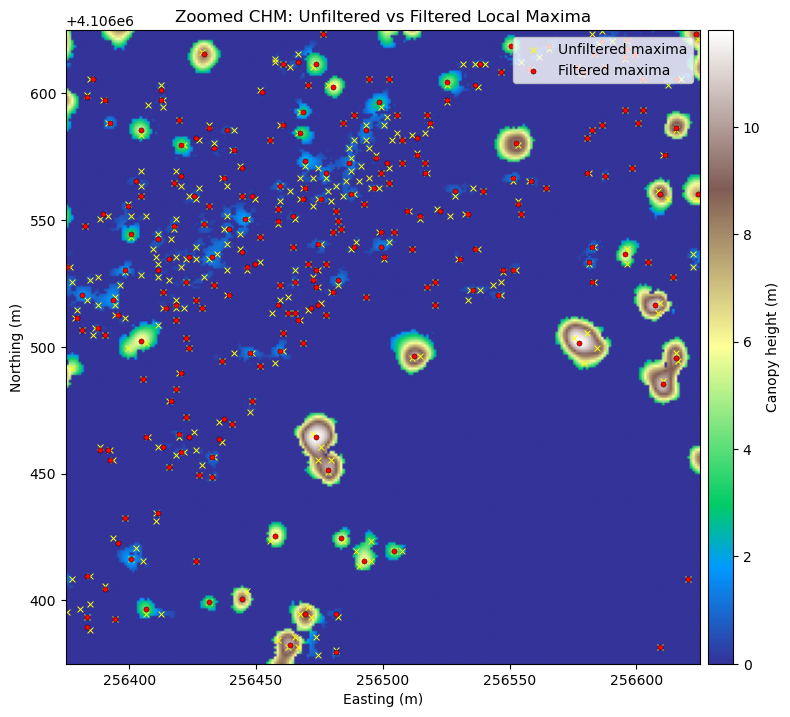
Looking at the overlap between the tree crowns and the local maxima from each method, you can see that filtering improves the results.
# Zoomed CHM section with unfiltered vs filtered local maxima overlay
from mpl_toolkits.axes_grid1 import make_axes_locatable

n_rows, n_cols = chm_array_smooth.shape

# Define a small window around the center of the tile
win_rows = min(250, n_rows)
win_cols = min(250, n_cols)
r0 = max(0, (n_rows // 2) - (win_rows // 2))
c0 = max(0, (n_cols // 2) - (win_cols // 2))
r1 = min(n_rows, r0 + win_rows)
c1 = min(n_cols, c0 + win_cols)

chm_zoom = chm_array_smooth[r0:r1, c0:c1]
local_zoom_filtered = local_maxi[r0:r1, c0:c1]
local_zoom_unfiltered = local_maxi_unfiltered[r0:r1, c0:c1]

# Use rasterio transform to get the true map extent for this zoom window
transform = chm_profile["transform"]
left, top = rio.transform.xy(transform, r0, c0, offset='ul')
right, bottom = rio.transform.xy(transform, r1 - 1, c1 - 1, offset='lr')
zoom_extent = (left, right, bottom, top)

# Convert local maxima row/col indices to map x/y for plotting
peak_rows_filtered, peak_cols_filtered = np.where(local_zoom_filtered)
peak_x_filtered, peak_y_filtered = rio.transform.xy(
    transform,
    peak_rows_filtered + r0,
    peak_cols_filtered + c0,
    offset='center'
    )

peak_rows_unfiltered, peak_cols_unfiltered = np.where(local_zoom_unfiltered)
peak_x_unfiltered, peak_y_unfiltered = rio.transform.xy(
    transform,
    peak_rows_unfiltered + r0,
    peak_cols_unfiltered + c0,
    offset='center'
    )

fig, ax = plt.subplots(figsize=(8, 8))
im = ax.imshow(chm_zoom, cmap='terrain', extent=zoom_extent, origin='upper')

if len(peak_x_unfiltered) > 0:
    ax.scatter(
        peak_x_unfiltered, peak_y_unfiltered, s=18, marker='x', c='yellow',
        linewidths=0.7, label='Unfiltered maxima'
        )
if len(peak_x_filtered) > 0:
    ax.scatter(
        peak_x_filtered, peak_y_filtered, s=14, c='red', edgecolors='black',
        linewidths=0.3, label='Filtered maxima'
        )

ax.set_title('Zoomed CHM: Unfiltered vs Filtered Local Maxima')
ax.set_xlabel('Easting (m)')
ax.set_ylabel('Northing (m)')
ax.legend(loc='upper right')

# Create a colorbar axis matched to the plot's y-axis height
divider = make_axes_locatable(ax)
cax = divider.append_axes('right', size='4%', pad=0.08)
fig.colorbar(im, cax=cax, label='Canopy height (m)')

plt.tight_layout()
#Identify all the maximum points
markers = ndi.label(local_maxi)[0]
Next, create a mask layer of all of the vegetation points so that the watershed segmentation will only occur on the trees and not extend into the surrounding ground points. Since 0 represent ground points in the CHM, setting the mask to 1 where the CHM is not zero will define the mask
#Create a CHM mask so the segmentation will only occur on the trees
chm_mask = chm_array_smooth
chm_mask[chm_array_smooth != 0] = 1
Watershed segmentation
As in a river system, a watershed is divided by a ridge that divides areas. Here our watershed are the individual tree canopies and the ridge is the delineation between each one.
See Basics of Image Processing - Watershed Segmentation for more information on this algorithm.
Next, carry out the watershed segmentation. This produces a raster of labels. First, we'll visualize the steps of the watershed segmentation process.
# Create a visualization showing the watershed segmentation process
fig, axes = plt.subplots(1, 2, figsize=(15, 5))

# Panel 1: Smoothed CHM with local maxima (markers)
im1 = axes[0].imshow(chm_array_smooth, cmap='viridis', extent=extent, origin='upper')
axes[0].scatter(chm_bounds.left + np.where(markers)[1] * (chm_bounds.right - chm_bounds.left) / chm_array_smooth.shape[1],
                chm_bounds.top - np.where(markers)[0] * (chm_bounds.top - chm_bounds.bottom) / chm_array_smooth.shape[0],
                c='red', s=30, marker='x', linewidths=2, label='Tree tops (markers)')
axes[0].set_title('Step 1: Smoothed CHM\nwith Tree Top Markers', fontsize=12, fontweight='bold')
axes[0].set_xlabel('X coordinate')
axes[0].set_ylabel('Y coordinate')
axes[0].legend(loc='upper right')
plt.colorbar(im1, ax=axes[0], label='Height (m)')

# Panel 2: CHM with vegetation mask
masked_chm = np.where(chm_mask, chm_array_smooth, np.nan)
im2 = axes[1].imshow(masked_chm, cmap='Greens', extent=extent, origin='upper')
axes[1].set_title('Step 2: Vegetation Mask\n(Algorithm only operates on vegetation)', fontsize=12, fontweight='bold')
axes[1].set_xlabel('X coordinate')
axes[1].set_ylabel('Y coordinate')
plt.colorbar(im2, ax=axes[1], label='Height (m)');
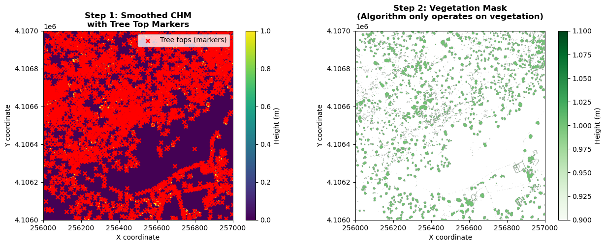
The visualization above shows the first two stages of watershed segmentation: 1. smoothing the CHM with detected tree top markers (red x's), and 2) the vegetation mask, showing only areas with trees included. The third and final step showing the resulting segments are shown after performing the watershed segmentation, in the next cell.
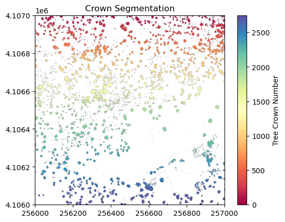
# Perform watershed segmentation
labels = watershed(chm_array_smooth, markers, mask=chm_mask)
labels_for_plot = labels.copy()
labels_for_plot = np.array(labels_for_plot,dtype = np.float32)
labels_for_plot[labels_for_plot==0] = np.nan
max_labels = np.max(labels)
# Plot the segments
plt.figure(4)
plt.imshow(labels_for_plot, cmap='Spectral', extent=extent, origin='upper', vmin=0, vmax=max_labels)
plt.title('Crown Segmentation')
plt.colorbar(label='Tree Crown Number')

plt.savefig(data_path+chm_name[0:-4]+'_Segmentation.png',
            dpi=300,orientation='landscape',
            bbox_inches='tight',pad_inches=0.1)

output_raster(
    os.path.join(data_path, 'labels.tif'),
    labels,
    chm_profile,
    dtype="int32",
    nodata=0
    )
Now collect several properties of the individual trees that will be used as predictor variables.
#Get the properties of each segment
tree_properties = regionprops(labels,chm_array)
Now we will get the predictor variables to match the (soon to be loaded) training data using the get_predictors function defined above. The first column is the segment ID, and the rest are the predictor variables, namely the tree area (pixels), major_axis_length, maximum height, minimum height, height percentiles (p50, p60, p70), and crown geometric volume percentiles (full and percentiles 50, 60, and 70).
predictors_chm = np.array([get_predictors(tree, chm_array, labels) for tree in tree_properties])
X = predictors_chm[:,1:]
tree_ids = predictors_chm[:,0]
np.shape(predictors_chm)
(2749, 12)
We now read the training data directly from GitHub. The CSV contains 12 columns: biomass (the target variable), followed by 11 predictor variables: area, major_axis_length, max_height, min_height, p50, p60, p70, full_crown, crown50, crown60, and crown70. Field-validated tree diameter (DBH) values are used to compute biomass using the formulas from Jenkins et al. (2003), while the remaining predictors were derived from the CHM by manually delineating tree crowns.
# Read training data from download path
training_data_csv = r'C:\NEON-Data-Skills\tutorials\Python\AOP\Lidar\lidar-applications\lidar-biomass\calc-biomass_py_files\SJER_Biomass_Training.csv'

# Alternatively, read training data directly from GitHub (raw CSV)
# training_data_csv = ('https://raw.githubusercontent.com/NEONScience/NEON-Data-Skills/'
#                      'main/tutorials/Python/AOP/Lidar/lidar-applications/'
#                      'lidar-biomass/calc-biomass_py_files/SJER_Biomass_Training.csv')

training_df = pd.read_csv(training_data_csv)

# Build per-column rounding: 0 dp for integer columns, 1 dp for float columns
decimals = {c: (0 if training_df[c].dtype == np.int64 else 1) for c in training_df.columns}

# Preview the data
print('Shape:', training_df.shape)
print()
print('First 5 rows:')
display(training_df.head().round(decimals))
print()
print('Summary statistics:')
display(training_df.describe().round(1))

# Extract numpy arrays for the model
biomass = training_df['biomass'].values
biomass_predictors = training_df.drop(columns=['biomass']).values
Shape: (42, 12)

First 5 rows:
| biomass | area | major_axis_length | max_height | min_height | p50 | p60 | p70 | full_crown | crown50 | crown60 | crown70 | |
|---|---|---|---|---|---|---|---|---|---|---|---|---|
| 0 | 14.2 | 23 | 5.6 | 9 | 5.4 | 8.2 | 8.4 | 8.5 | 54.1 | 48.7 | 50.5 | 51.5 |
| 1 | 7643.4 | 47 | 10.9 | 12 | 6.7 | 10.4 | 10.7 | 10.8 | 159.0 | 146.0 | 151.0 | 154.0 |
| 2 | 889.0 | 16 | 12.4 | 11 | 7.0 | 9.8 | 10.1 | 10.2 | 39.5 | 34.8 | 37.0 | 37.3 |
| 3 | 456.9 | 26 | 10.3 | 11 | 5.8 | 8.6 | 9.0 | 9.2 | 68.6 | 55.5 | 60.8 | 62.6 |
| 4 | 296.7 | 5 | 11.8 | 11 | 8.3 | 10.6 | 10.7 | 10.8 | 9.4 | 8.4 | 8.6 | 8.7 |
Summary statistics:
| biomass | area | major_axis_length | max_height | min_height | p50 | p60 | p70 | full_crown | crown50 | crown60 | crown70 | |
|---|---|---|---|---|---|---|---|---|---|---|---|---|
| count | 42.0 | 42.0 | 42.0 | 42.0 | 42.0 | 42.0 | 42.0 | 42.0 | 42.0 | 42.0 | 42.0 | 42.0 |
| mean | 2644.0 | 33.5 | 8.4 | 9.2 | 5.1 | 7.5 | 7.8 | 8.0 | 99.9 | 85.6 | 90.1 | 93.2 |
| std | 4851.6 | 29.3 | 3.4 | 3.6 | 1.8 | 2.7 | 2.8 | 2.9 | 129.5 | 113.3 | 118.5 | 122.2 |
| min | 14.2 | 3.0 | 3.6 | 5.0 | 2.1 | 2.8 | 2.9 | 3.3 | 1.4 | 0.3 | 0.5 | 0.8 |
| 25% | 240.1 | 15.2 | 6.1 | 7.0 | 4.0 | 5.7 | 5.8 | 6.0 | 26.2 | 23.5 | 24.0 | 24.7 |
| 50% | 659.4 | 23.0 | 7.5 | 8.5 | 5.0 | 7.0 | 7.2 | 7.3 | 47.4 | 38.2 | 41.0 | 42.3 |
| 75% | 2791.3 | 41.2 | 10.7 | 11.0 | 5.7 | 8.6 | 9.0 | 9.2 | 88.4 | 72.2 | 78.4 | 82.8 |
| max | 25968.4 | 118.0 | 18.2 | 21.0 | 11.8 | 15.5 | 16.0 | 16.5 | 627.0 | 553.0 | 574.0 | 591.0 |
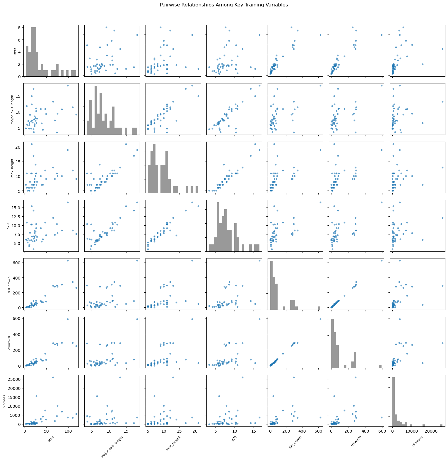
Let's inspect the training data by making some pairwise plots.
# Inspect pairwise relationships among training-data columns
column_names = training_df.columns.tolist()
# Summary table
summary = training_df.describe().round(1)
print('Column summary (min, max, mean, std):')
for name in column_names:
mn = summary.loc['min', name]
mx = summary.loc['max', name]
mu = summary.loc['mean', name]
sd = summary.loc['std', name]
print(f'{name:>16s}: min={mn:10.1f}, max={mx:10.1f}, mean={mu:10.1f}, std={sd:10.1f}')
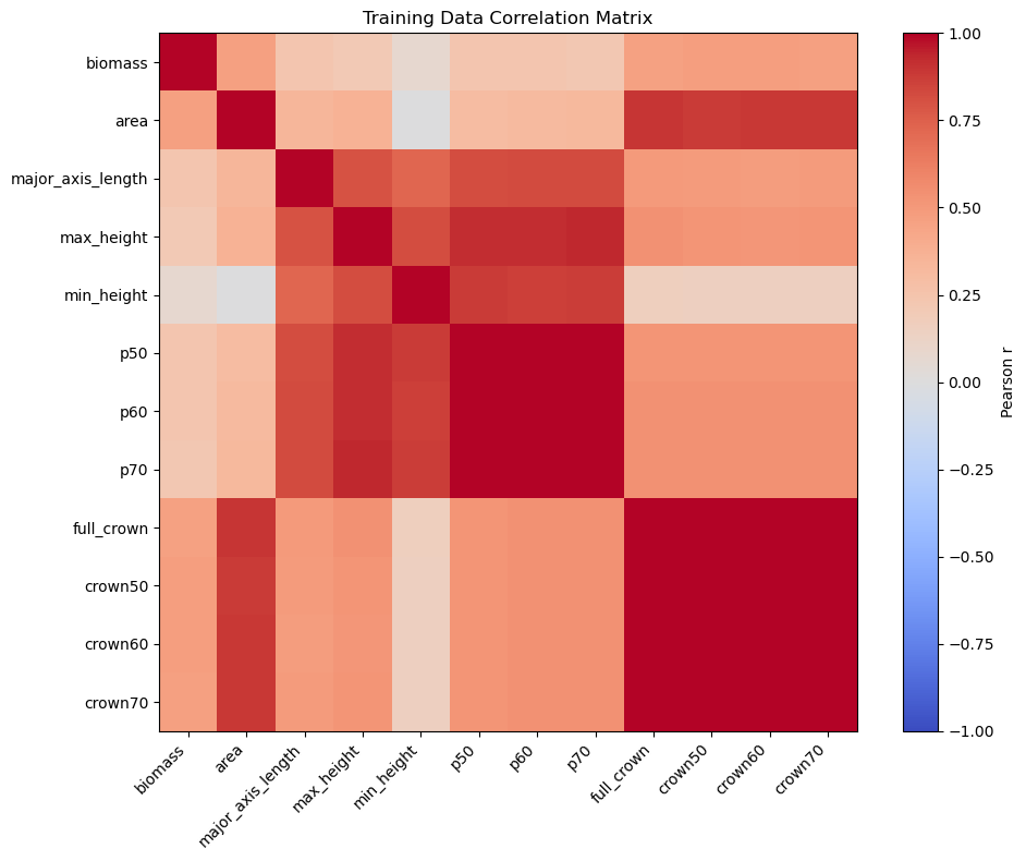
# Plot 1: correlation heatmap (all columns)
corr = training_df.corr(numeric_only=True)
fig, ax = plt.subplots(figsize=(10, 8))
im = ax.imshow(corr, cmap='coolwarm', vmin=-1, vmax=1)
ax.set_xticks(np.arange(len(corr.columns)))
ax.set_yticks(np.arange(len(corr.columns)))
ax.set_xticklabels(corr.columns, rotation=45, ha='right')
ax.set_yticklabels(corr.columns)
ax.set_title('Training Data Correlation Matrix')
plt.colorbar(im, ax=ax, label='Pearson r')
plt.tight_layout()
# Plot 2: scatter matrix style plot (key variables)
plot_columns = [
'area', 'major_axis_length', 'max_height', 'p70',
'full_crown', 'crown70', 'biomass'
]
plot_df = training_df[plot_columns]
n = len(plot_columns)
fig, axes = plt.subplots(n, n, figsize=(2.2 * n, 2.2 * n), squeeze=False)
for i in range(n):
for j in range(n):
ax = axes[i, j]
if i == j:
ax.hist(plot_df.iloc[:, j], bins=20, color='gray', alpha=0.8)
else:
ax.scatter(plot_df.iloc[:, j], plot_df.iloc[:, i], s=10, alpha=0.6, color='tab:blue')
if i == n - 1:
ax.set_xlabel(plot_columns[j], fontsize=8, rotation=45)
else:
ax.set_xticklabels([])
if j == 0:
ax.set_ylabel(plot_columns[i], fontsize=8)
else:
ax.set_yticklabels([])
fig.suptitle('Pairwise Relationships Among Key Training Variables', y=1.02)
plt.tight_layout()
Column summary (min, max, mean, std):
         biomass: min=      14.2, max=   25968.4, mean=    2644.0, std=    4851.6
            area: min=       3.0, max=     118.0, mean=      33.5, std=      29.3
major_axis_length: min=       3.6, max=      18.2, mean=       8.4, std=       3.4
      max_height: min=       5.0, max=      21.0, mean=       9.2, std=       3.6
      min_height: min=       2.1, max=      11.8, mean=       5.1, std=       1.8
             p50: min=       2.8, max=      15.5, mean=       7.5, std=       2.7
             p60: min=       2.9, max=      16.0, mean=       7.8, std=       2.8
             p70: min=       3.3, max=      16.5, mean=       8.0, std=       2.9
      full_crown: min=       1.4, max=     627.0, mean=      99.9, std=     129.5
         crown50: min=       0.3, max=     553.0, mean=      85.6, std=     113.3
         crown60: min=       0.5, max=     574.0, mean=      90.1, std=     118.5
         crown70: min=       0.8, max=     591.0, mean=      93.2, std=     122.2
Random Forest classifiers
We can then define parameters of the Random Forest classifier and fit the predictor variables from the training data to the Biomass estimates.
#Define parameters for the Random Forest Regressor
max_depth = 30

#Define regressor settings
regr_rf = RandomForestRegressor(max_depth=max_depth, random_state=2)

#Fit the biomass to regressor variables
regr_rf.fit(biomass_predictors,biomass)
We will now apply the Random Forest model to the predictor variables to estimate biomass
#Apply the model to the predictors
estimated_biomass = regr_rf.predict(X)
To output a raster, pre-allocate (copy) an array from the labels raster, then cycle through the segments and assign the biomass estimate to each individual tree segment.
#Set an out raster with the same size as the labels
biomass_map =  np.array((labels),dtype=float)
#Assign the appropriate biomass to the labels
biomass_map[biomass_map==0] = np.nan
for tree_id, biomass_of_tree_id in zip(tree_ids, estimated_biomass):
    biomass_map[biomass_map == tree_id] = biomass_of_tree_id
Calculate Biomass
Collect some of the biomass statistics and then plot the results and save an output geotiff.
#Get biomass stats for plotting
mean_biomass = np.mean(estimated_biomass)
std_biomass = np.std(estimated_biomass)
min_biomass = np.min(estimated_biomass)
sum_biomass = np.sum(estimated_biomass)
print('Sum of above ground biomass (AGB) is',round(sum_biomass,1),'kg')
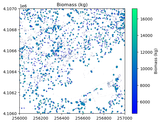
# Plot the biomass
plt.figure(5)
plt.imshow(
biomass_map,
cmap='winter',
extent=extent,
origin='upper',
vmin=min_biomass + std_biomass,
vmax=mean_biomass + std_biomass * 3
)
plt.title('Biomass (kg)')
plt.colorbar(label='Biomass (kg)')
# Save the biomass figure; use the same name as the original file, but replace CHM with Biomass
plt.savefig(os.path.join(data_path,chm_name.replace('CHM.tif','Biomass.png')),
dpi=300,orientation='landscape',
bbox_inches='tight',
pad_inches=0.1)
# Write biomass geotiff with rasterio
output_raster(
os.path.join(data_path, chm_name.replace('CHM.tif','Biomass.tif')),
biomass_map,
chm_profile,
dtype="float32",
nodata=np.nan
)
Sum of above ground biomass (AGB) is 10515682.7 kg
Friday: Applications in Remote Sensing
Today, you will use all of the skills you've learned at the Institute to work on a group project that uses NEON or related data!
Learning Objectives
During this activity you will:
- Apply the skills that you have learned to process data using efficient coding practices.
- Apply your understanding of remote sensing data and use it to address a science question of your choice.
- Implement version control and collaborate with your colleagues through the GitHub platform.
| Time | Topic | Location |
|---|---|---|
| 9:00 | Groups begin work on capstone projects | Breakout rooms |
| Instructors available on an as needed basis for consultation & help | ||
| 12:00 | Lunch | Classroom/Patio |
| Groups continue to work on capstone projects | Breakout rooms | |
| 16:30 | End of day wrap up | Classroom |
| 18:00 | Time to leave the building (if group opts to work after wrap up) |
Additional Resources
Saturday: Capstone Projects
| Time | Topic | Instructor |
|---|---|---|
| 9:00 | Presentations Start | |
| 11:30 | Final Questions & Institute Debrief | |
| 12:00 | Lunch | |
| 13:00 | End |