Tutorial
Linking NEON aquatic observational and instrument data to answer critical questions in aquatic ecology at the continental scale
Last Updated: May 15, 2026
Learning Objectives
After completing this activity, you will be able to:
- Download NEON AIS and AOS data using the
neonUtilitiespackage. - Understand downloaded data packages and load them into R for analyses.
- Understand the similarities and linkages between different NEON data products.
- Join data sets within and between data products by standardized variables.
- Plot instrumented and observational data in the same plotting field.
Things You'll Need To Complete This Tutorial
To complete this tutorial you will need R (version >3.4) and, preferably, RStudio loaded on your computer.
Install R Packages
- neonUtilities: Basic functions for accessing NEON data
- neonOS: Basic data wrangling for NEON Observational Data
- tidyverse: Collection of R packages designed for data science
- plotly: Tool for creating interactive, web-based visualizations
- vegan: Functions for analyzing ecological data
- base64enc: Tools for base64 encoding
These packages are on CRAN and can be installed by
install.packages().
Additional Resources
Introduction
Tutorial Overview
This tutorial covers downloading NEON Aquatic Instrument Subsystem (AIS) and
Aquatic Observation Subsystem (AOS) data products using the neonUtilities R
package, as well as basic instruction in beginning to explore and work with the
downloaded data. This includes navigating data packages documentation,
summarizing data for plotting and analysis, combining data within and between
data products, and visualizing AIS and AOS data separately and together.
Helpful Links
Getting started with NEON data: https://www.neonscience.org/resources/getting-started-neon-data-resources
Contact us form: https://www.neonscience.org/about/contact-us
Teaching Modules: https://www.neonscience.org/resources/learning-hub/teaching-modules
QUBES modules: https://qubeshub.org/community/groups/neon/educational_resources
EDDIE modules : https://serc.carleton.edu/eddie/macrosystems/index.html
Spatial data and maps: https://neon.maps.arcgis.com/home/index.html
NEON data portal: https://data.neonscience.org/
Download Files and Load Directly to R: loadByProduct()
The most popular function in neonUtilities is loadByProduct().
This function downloads data from the NEON API, merges the site-by-month
files, and loads the resulting data tables into the R environment,
assigning each data type to the appropriate R class. This is a popular
choice because it ensures you're always working with the most up-to-date data,
and it ends with ready-to-use tables in R. However, if you use it in
a workflow you run repeatedly, keep in mind it will re-download the
data every time.
Before we get the NEON data, we need to install (if not already done) and load the neonUtilities R package, as well as other packages we will use in the analysis.
# # install neonUtilities package if you have not yet.

# install.packages("neonUtilities")

# install.packages("neonOS")

# install.packages("tidyverse")

# install.packages("plotly")

# install.packages("vegan")

# install.packages("base64enc")

# install.packages("htmlwidgets")

# install.packages("htmltools")
Load Packages Into Workspace
# load required packages

library(neonUtilities)

library(neonOS)

library(tidyverse)

library(plotly)

library(vegan)

library(base64enc)

library(htmlwidgets)

library(htmltools)
Inputs: loadByProduct()
The inputs to loadByProduct() control which data to download and how
to manage the processing. The following are frequently used inputs:
-
dpID: the data product ID, e.g. DP1.20288.001 -
site: defaults to "all", meaning all sites with available data; can be a vector of 4-letter NEON site codes, e.g.c("MART","ARIK","BARC"). -
startdateandenddate: defaults to NA, meaning all dates with available data; or a date in the form YYYY-MM, e.g. 2017-06. Since NEON data are provided in month packages, finer scale querying is not available. Both start and end date are inclusive. -
package: either basic or expanded data package. Expanded data packages generally include additional information about data quality, such as individual quality flag test results. Not every NEON data product has an expanded package; if the expanded package is requested but there isn't one, the basic package will be downloaded. -
release: The data release to be downloaded; either 'current' or the name of a release, e.g. 'RELEASE-2026'. 'current' returns provisional data in addition to the most recent release. To download only provisional data, use release='PROVISIONAL'. Defaults to 'current'. See https://www.neonscience.org/data-samples/data-management/data-revisions-releases for more information. -
include.provisional: Should provisional data be included in the downloaded files? Defaults to F. -
timeIndex: defaults to "all", to download all data; or the number of minutes in the averaging interval. See example below; only applicable to IS data. -
check.size: T or F; should the function pause before downloading data and warn you about the size of your download? Defaults to T; if you are using this function within a script or batch process you will want to set this to F. -
token: this allows you to input your NEON API token to obtain faster downloads. Learn more about NEON API tokens in the Using an API Token when Accessing NEON Data with neonUtilities tutorial.
There are additional inputs you can learn about in the Use the neonUtilities R Package to Access NEON Data tutorial.
The dpID is the data product identifier of the data you want to
download. The DPID can be found on the
Explore Data Products page.
It will be in the form DP#.#####.###. For this tutorial, we'll use some data products collected in NEON's aquatics program:
- DP1.20120.001: Macroinvertebrate collection
- DP4.00130.001: Continuous discharge
NEON Aquatic Sites
Now it's time to consider the NEON field site of interest. If not specified, the default will download a data product from all sites. The following are 4-letter site codes for NEON's 34 aquatics sites:
- ARIK=Arikaree River CO
- BARC=Barco Lake FL
- BIGC=Upper Big Creek CA
- BLDE=Black Deer Creek WY
- BLUE=Blue River OK
- BLWA=Black Warrior River AL
- CARI=Caribou Creek AK
- COMO=Como Creek CO
- CRAM=Crampton Lake WI
- CUPE=Rio Cupeyes PR
- FLNT=Flint River GA
- GUIL=Rio Yahuecas PR
- HOPB=Lower Hop Brook MA
- KING=Kings Creek KS
- LECO=LeConte Creek TN
- LEWI=Lewis Run VA
- LIRO=Little Rock Lake WI
- MART=Martha Creek WA
- MAYF=Mayfield Creek AL
- MCDI=McDiffett Creek KS
- MCRA=McRae Creek OR
- OKSR=Oksrukuyik Creek AK
- POSE=Posey Creek VA
- PRIN=Pringle Creek TX
- PRLA=Prairie Lake ND
- PRPO=Prairie Pothole ND
- REDB=Red Butte Creek UT
- SUGG=Suggs Lake FL
- SYCA=Sycamore Creek AZ
- TECR=Teakettle Creek CA
- TOMB=Lower Tombigbee River AL
- TOOK=Toolik Lake AK
- WALK=Walker Branch TN
- WLOU=West St Louis Creek CO
With the exception of the case studies, each section of the tutorial can be run on any number of sites. Choose which sites you would like to explore by creating a vector of 4-letter NEON site codes.
# create vector of site names to use in loadByProduct()

siteList <- c("CUPE", "GUIL")
Downloading Data By Water Year
We will focus our exercise on data collected by water year. A water year is
defined as October 1 through September 30. For example, water year 2022 spans
2021-10-01 - 2022-09-30. Set the start and end water year you would like to
explore, and the code will format the dates for querying data using
neonUtilities.
# set the start and end water years to explore

startWY <- 2022

endWY <- 2024


# DO NOT EDIT - format dates for neonUtilities

startWY_query <- paste0(startWY-1, "-10")

endWY_query <- paste0(endWY, "-09")
Now let us download our data. If you are not using a NEON token to download your
data, neonUtilities will ignore the token input. We set check.size=F so
that the script runs well but remember you always want to check your download
size first. For this exercise, we will focus on the following data products:
AIS Data Products:
- Continuous discharge (DP4.00130.001)
AOS Data Products:
- Macroinvertebrate collection (DP1.20120.001)
Download AOS Data Products
# download data of interest - AOS - Macroinvertebrate collection

inv <- loadByProduct(dpID="DP1.20120.001",
                     site=siteList,
                     startdate=startWY_query,
                     enddate=endWY_query,
                     package="expanded",
                     release="current",
                     include.provisional=T,
                     token=Sys.getenv("NEON_TOKEN"),
                     check.size=F)
Files Associated with Downloads
The data we've downloaded comes as an object that is a named list of objects.
To work with each of them, select them from the list using the $ operator.
# view all components of the list

names(inv)

##  [1] "categoricalCodes_20120"      "citation_20120_RELEASE-2026" "inv_fieldData"               "inv_persample"
##  [5] "inv_taxonomyProcessed"       "inv_taxonomyRaw"             "issueLog_20120"              "readme_20120"
##  [9] "validation_20120"            "variables_20120"
We can see that there are at least 9 objects in the downloaded macroinvertebrate collection data.
- 4 dataframes of data:
-
inv_fieldData -
inv_persample -
inv_taxonomyProcessed -
inv_taxonomyRaw
-
- 5 metadata files:
-
categoricalCodes_20120 -
issueLog_20120 -
readme_20120 -
validation_20120 -
variables_20120
-
- At least 1 data citation file:
- Example files:
-
citation_20120_PROVISIONAL -
citation_20120_RELEASE-2026
-
- Example files:
If you'd like you can use the $ operator to assign an object from an item in
the list. If you prefer to extract each table from the list and work with it as
independent objects, which we will do, you can use the list2env() function.
# unlist the variables and add to the global environment

list2env(inv, envir=.GlobalEnv)

## <environment: R_GlobalEnv>
Explore: Data Citations
Citing sources correctly helps the NEON user community maintain transparency, openness, and trust, while also providing a benefit of being able to track the impact of NEON on scientific research. Thus, each download of NEON data comes with proper citations custom to to the download that align with NEON's data citation guidelines
# view formatted citations for DP1.20120.001 download

# locate any citation files and print them in the console

citationFiles <- names(inv)[grepl("citation", names(inv))]

for(c in citationFiles){cat(get(c))}

## @misc{https://doi.org/10.48443/hp56-s582,
##   doi = {10.48443/HP56-S582},
##   url = {https://data.neonscience.org/data-products/DP1.20120.001/RELEASE-2026},
##   author = {{National Ecological Observatory Network (NEON)}},
##   keywords = {diversity, taxonomy, community composition, species composition, population, aquatic, benthic, macroinvertebrates, invertebrates, abundance, streams, lakes, rivers, wadeable streams, material samples, archived samples, biodiversity},
##   language = {en},
##   title = {Macroinvertebrate collection (DP1.20120.001)},
##   publisher = {National Ecological Observatory Network (NEON)},
##   year = {2026}
## }
Explore: Metadata
- categoricalCodes_xxxxx: Some variables in the data tables are published as strings and constrained to a standardized list of values (LOV). This file shows all the LOV options for variables published in this data product.
- issueLog_xxxxx: Issues that may impact data quality, or changes to a data product that affects all sites, are reported in this file.
- readme_xxxxx: The readme file provides important information relevant to the data product and the specific instance of downloading the data.
- validation_xxxxx: If any fields require validation prior to publication, those validation rules are reported in this table
- variables_xxxxx: This file contains all the variables found in the associated data table(s). This includes full definitions, units, and other important information.
Let's view the full variables file data frame to explore details on tables and fields in this data product.
# view the entire dataframe in your R environment

view(variables_20120)
Explore: Dataframes
There will always be one or more dataframes that include the primary data of the data product you downloaded. Multiple dataframes are available when there are related datatables for a single data product.
# view the entire dataframe in your R environment

view(inv_fieldData)
Download AIS Data Products
# download data of interest - AIS - Continuous discharge

csd <- loadByProduct(dpID="DP4.00130.001",
                     site=siteList,
                     startdate=startWY_query,
                     enddate=endWY_query,
                     package="basic",
                     release= "current",
                     include.provisional=T,
                     token=Sys.getenv("NEON_TOKEN"),
                     check.size=F)
Let's see what files are included with an AIS data product download
# view all components of the list

names(csd)

## [1] "categoricalCodes_00130"      "citation_00130_RELEASE-2026" "csd_15_min"                  "issueLog_00130"
## [5] "readme_00130"                "science_review_flags_00130"  "sensor_positions_00130"      "variables_00130"
This AIS data product contains 1 data table available in the basic package:
-
csd_15_min- Continuous discharge (streamflow) data at a 15 minute interval
- Being a Level 4 data product, this data has been cleaned and gap-filled
Additionally, there are a couple of metadata file types included in AIS data product downloads that are not included in AOS data product downloads:
- sensor_postions_xxxxx: This file contains information about the coordinates of each sensor, relative to a reference location.
- science_review_flags_xxxxx: This file contains information on quality flags added to the data following expert review for data that are determined to be suspect due to known adverse conditions not captured by automated flagging.
Let's unpack the AIS data product to the environment:
# unlist the variables and add to the global environment

list2env(csd, .GlobalEnv)

## <environment: R_GlobalEnv>
Wrangling AOS Data
The neonOS R package was developed to aid in wrangling NEON Observational
Subsystem (OS) data products. Two functions used in this exercise are:
-
removeDups() -
joinTableNEON()
Removing Duplicates from OS Data
Duplicates can arise in data, but the removeDups() function identifies
duplicates in a data table based on primary key information reported in the
variables_xxxxx files included in each data download.
Let's check for duplicates in macroinvertebrate collection data
# what are the primary keys in inv_fieldData?

cat("Primary keys in inv_fieldData are:",
    paste(variables_20120$fieldName[
      variables_20120$table=="inv_fieldData"
      &variables_20120$primaryKey=="Y"
    ],
    collapse=", ")
    )
Primary keys in inv_fieldData are: namedLocation, eventID, sampleID, sampleCode, habitatType, samplerType, sampleNumber
# identify duplicates in inv_fieldData

inv_fieldData_dups <- removeDups(inv_fieldData,
                                 variables_20120)

cat("There are",
    sum(inv_fieldData_dups$duplicateRecordQF%in%c(1, 2)),
    "duplicate records in 'inv_fieldData'")
There are 0 duplicate records in 'inv_fieldData'
# what are the primary keys in inv_persample?

cat("Primary keys in inv_persample are:",
    paste(variables_20120$fieldName[
      variables_20120$table=="inv_persample"
      &variables_20120$primaryKey=="Y"
    ],
    collapse=", ")
    )
Primary keys in inv_persample are: sampleID, sampleCode
# identify duplicates in inv_persample

inv_persample_dups <- removeDups(inv_persample,
                                 variables_20120)

cat("There are",
    sum(inv_persample_dups$duplicateRecordQF%in%c(1, 2)),
    "duplicate records in 'inv_persample'")
There are 0 duplicate records in 'inv_persample'
# what are the primary keys in inv_taxonomyProcessed?

cat("Primary keys in inv_taxonomyProcessed are:",
    paste(variables_20120$fieldName[
      variables_20120$table=="inv_taxonomyProcessed"
      &variables_20120$primaryKey=="Y"
    ],
    collapse=", ")
    )
Primary keys in inv_taxonomyProcessed are: sampleID, sampleCode, slideID, slideCode, scientificName, morphospeciesID, invertebrateLifeStage, sizeClass, sizeCategory, immatureSpecimen, indeterminateSpecies, taxonRankQualifier, sampleCondition, distinctTaxon, identificationRemarks
# identify duplicates in inv_taxonomyProcessed

inv_taxonomyProcessed_dups <- removeDups(inv_taxonomyProcessed,
                                         variables_20120)

cat("There are",
    sum(inv_fieldData_dups$duplicateRecordQF%in%c(1, 2)),
    "duplicate records in 'inv_taxonomyProcessed'")
There are 0 duplicate records in 'inv_taxonomyProcessed'
Thankfully, there are no duplicates in any of the AOS tables used in this exercise!
Joining OS Data Tables
Every NEON data product comes with a Quick Start Guide (QSG). The QSGs contain basic information to help users familiarize themselves with the data products, including description of the data contents, data quality information, common calculations or transformations, and, where relevant, algorithm description and/or table joining instructions.
The QSG for Macroinvertebrate collection can be found on the data product landing page
The joinTableNEON() function uses the table joining information in the
QSG to quickly join two related NEON data tables from the same data product
# join inv_fieldData and inv_taxonomyProcessed

inv_fieldTaxJoined <- joinTableNEON(inv_fieldData, inv_taxonomyProcessed)
Now, with field and taxonomy data joined. Individual taxon identifications are easily linked to field data such as collection latitude/longitude, habitat type, sampler type, and substratum class.
Plot Data
Now that we have wrangled the data a bit to make it easier to work with, let's make some initial plots to see the AOS and AIS data separately before we begin to investigate questions that involve integrating the data.
AOS Macroinvertebrate abundance and richness
First, we remove the records collected outside of normal sampling bouts as a grab sample. In cases where the NEON field ecologists see interesting organisms that would not be captured using standard field sampling methods, they can collect a grab sample to be identified by the expert taxonomists.
Next, we calculate macroinvertebrate abundance per square meter and taxon richness per sampling bout. This allows us to compare macroinvertebrate data among different samplerTypes and habitatTypes.
We use the vegan R package to calculate richness, evenness, and both the
Shannon and Simpson biodiversity indicies in this exercise. Though we only
focus on richness in the plots, users are encouraged to alter the variables
to view other indices. For a more detailed dive into NEON biodiversity analyses,
see the following NEON tutorial:
Explore and work with NEON biodiversity data from aquatic ecosystems
Sampler types (e.g., surber, hand corer, kicknet) are strongly associated with habitat (i.e., riffle, run, pool) and substrata. Data users should look at the data to determine how they want to discriminate between sampler or habitat type.
For this exercise, we split abundance and richness by habitatType. To split
instead by samplerType, simply do a find+replace of
'habitatType' -> 'samplerType' throughout the code.
# show breakdown of sampler type by habitat type at each site

sampler_habitat_summ <- inv_fieldTaxJoined%>%
  distinct(siteID, samplerType, habitatType)

sampler_habitat_summ

##   siteID samplerType habitatType
## 1   CUPE      surber      riffle
## 2   CUPE      surber         run
## 3   GUIL        hess        pool
## 4   GUIL      surber      riffle
## 5   GUIL        hess         run
Let's wrangle invertebrate data and calculate abundance per square meter.
# using the `tidyverse` collection, we can clean the data in one piped function

inv_abundance_summ <- inv_fieldTaxJoined%>%
  # remove events when no samples were collected (samplingImpractical)
  # remove samples not associated with a bout
  filter(is.na(samplingImpractical)&!grepl("GRAB|BRYOZOAN", sampleID))%>%

  # calculate abundance (individuals per m2^)
  mutate(abun_M2=estimatedTotalCount/benthicArea)%>%

  # clean `collectDate` column header
  rename(collectDate=collectDate.x)%>%

  # first, group including `sampleID` and calculate total abundance per sample
  group_by(siteID, collectDate, eventID, sampleID, habitatType, boutNumber)%>%
  summarize(abun_M2_sum=sum(abun_M2, na.rm=TRUE))%>%

  # second, group excluding `sampleID` to summarize by each bout (`eventID`)
  group_by(siteID, collectDate, eventID, habitatType, boutNumber)%>%

  # summarize to get mean (+/- se) abundance by bout and sampler type
  summarise(across(abun_M2_sum,
                   list(mean=mean, sd=sd,
                        se=~sd(.x, na.rm=TRUE)/sqrt(n())),
                   .names="{.col}_{.fn}"))%>%

  # get categorical variable to sort bouts chronologically
  mutate(year=substr(eventID, 6, 9),
         yearBout=paste(year, "Bout", boutNumber, sep="."))
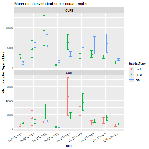
Plot abundance per square meter split by site, bout, and habitat type.
# produce stacked plot to show trends within and across sites

inv_abundance_summ%>%
  ggplot(aes(fill=habitatType, color=habitatType,
             y=abun_M2_sum_mean, x=yearBout))+
  geom_point(position=position_dodge(0.5), size=2)+
  geom_errorbar(aes(ymin=abun_M2_sum_mean-abun_M2_sum_se,
                    ymax=abun_M2_sum_mean+abun_M2_sum_se),
                width=0.4, alpha=3.0, linewidth=1,
                position=position_dodge(0.5))+
  facet_wrap(~siteID, ncol=1, scales="free_y")+
  theme(axis.text.x=element_text(size=10, angle=30, hjust=1, vjust=1))+
  labs(title="Mean macroinvertebrates per square meter",
       y="Abundance Per Square Meter",
       x="Bout")
Now, let's wrangle the data in a different way to prepare for diversity analysis
using the vegan package.
inv_richness_clean <- inv_fieldTaxJoined%>%
  # remove events when no samples were collected (samplingImpractical)
  # remove samples not associated with a bout
  filter(is.na(samplingImpractical)&!grepl("GRAB|BRYOZOAN", sampleID))%>%
  # clean `collectDate` column header
  rename(collectDate=collectDate.x)

# extract sample metadata

inv_sample_info <- inv_richness_clean%>%
  select(sampleID, domainID, siteID, namedLocation,
         collectDate, eventID, boutNumber,
         habitatType, samplerType, benthicArea)%>%
  distinct()

# filter out rare taxa: only observed 1 (singleton) or 2 (doubleton) times

inv_rare_taxa <- inv_richness_clean%>%
  distinct(sampleID, acceptedTaxonID, scientificName)%>%
  group_by(scientificName)%>%
  summarize(occurrences=n())%>%
  filter(occurrences > 2)

# filter richness table based on taxon list excluding singletons and doubletons

inv_richness_clean <- inv_richness_clean %>%
  filter(scientificName%in%inv_rare_taxa$scientificName)

# create a matrix of taxa by sampleID

inv_richness_clean_wide <- inv_richness_clean %>%
  # subset to unique combinations of `sampleID` and `scientificName`
  distinct(sampleID, scientificName, .keep_all=T)%>%

  # remove any records with no abundance data
  mutate(abun_M2=estimatedTotalCount/benthicArea)%>%
  filter(!is.na(abun_M2))%>%

  # pivot to wide format, sum multiple counts per sampleID
  pivot_wider(id_cols=sampleID,
              names_from=scientificName,
              values_from=abun_M2,
              values_fill=list(abun_M2=0),
              values_fn=list(abun_M2=sum)) %>%
  column_to_rownames(var="sampleID") %>%

  #round to integer so that vegan functions will run
  round()

# code check - check col and row sums

# mins should all be > 0 for further analysis in vegan

if(colSums(inv_richness_clean_wide) %>% min()==0){
  stop("Column sum is 0: do not proceed with richness analysis!")
}

if(rowSums(inv_richness_clean_wide) %>% min()==0){
  stop("Row sum is 0: do not proceed with richness analysis!")
}
Use the vegan package to calculate diversity indices.
# calculate richness

inv_richness <- as.data.frame(
  specnumber(inv_richness_clean_wide)
  )

names(inv_richness) <- "richness"

inv_richness_stats <- estimateR(inv_richness_clean_wide)

# calculate evenness

inv_evenness <- as.data.frame(
  diversity(inv_richness_clean_wide)/log(specnumber(inv_richness_clean_wide))
  )

names(inv_evenness) <- "evenness"

# calculate shannon index

inv_shannon <- as.data.frame(
  diversity(inv_richness_clean_wide, index="shannon")
  )

names(inv_shannon) <- "shannon"

# calculate simpson index

inv_simpson <- as.data.frame(
  diversity(inv_richness_clean_wide, index="simpson")
  )

names(inv_simpson) <- "simpson"

# create a single data frame

inv_diversity_indices <- cbind(inv_richness,
                               inv_evenness,
                               inv_shannon,
                               inv_simpson)

# bring in the metadata table created earlier

inv_diversity_indices <- left_join(rownames_to_column(inv_diversity_indices),
                                   inv_sample_info,
                                   by=c("rowname"="sampleID")) %>%
  rename(sampleID=rowname)

# create summary table for plotting

inv_diversity_summ <- inv_diversity_indices%>%
  pivot_longer(c(richness, evenness, shannon, simpson),
               names_to="indexName",values_to="indexValue")%>%
  group_by(siteID, collectDate, eventID, habitatType, boutNumber, indexName)%>%
  summarize(mean=mean(indexValue),
            n=n(),
            sd=sd(indexValue),
            se=sd/sqrt(n))%>%
  mutate(year=substr(eventID, 6, 9),
         yearBout=paste(year, "Bout", boutNumber, sep="."))
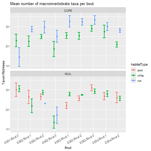
Plot taxon richness split by site, bout, and habitat type.
# produce plot to show trends within and across sites

inv_diversity_summ%>%
  filter(indexName=="richness")%>%
  ggplot(aes(fill=habitatType, color=habitatType, y=mean, x=yearBout))+
  geom_point(position=position_dodge(0.5), size=2)+
  geom_errorbar(aes(ymin=mean-se, ymax=mean+se),
                width=0.4, alpha=3.0, linewidth=1,
                position=position_dodge(0.5))+
  facet_wrap(~siteID, ncol=1)+
  theme(axis.text.x=element_text(size=10, angle=30,
                                 hjust=1, vjust=1))+
  labs(title="Mean number of macroinvertebrate taxa per bout",
       y= "Taxon Richness", x="Bout")
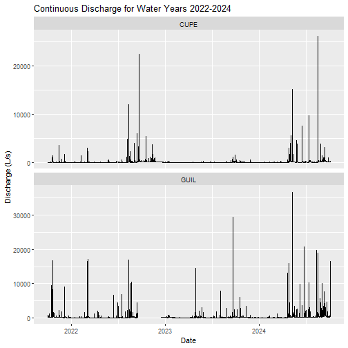
AIS Continuous discharge timseries
Now, let's visualize the cleaned and gap-filled continuous discharge timeseries for the two NEON D04 sites.
# plot with discharge in linear scale

csd_15_min%>%
  ggplot(aes(x=startDateTime, y=dischargeContinuous))+
  geom_line()+
  facet_wrap(~siteID, ncol=1, scales="free_y")+
  labs(title="Continuous Discharge for Water Years 2022-2024",
       y= "Discharge (L/s)", x="Date")
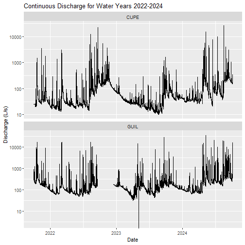
# plot with discharge in log scale

csd_15_min%>%
  ggplot(aes(x=startDateTime, y=dischargeContinuous))+
  geom_line()+
  facet_wrap(~siteID, ncol=1, scales="free_y")+
  scale_y_log10()+
  labs(title="Continuous Discharge for Water Years 2022-2024",
       y= "Discharge (L/s)", x="Date")
Visualize AOS and AIS Data Together
Next, we will use the R package plotly to make fun interactive plots allowing
us to view AOS and AIS data in the same plotting field. There is a
lot of code here to correctly format the plot in a way to provide as much info
and be as interactive as possible in a single plotting field.
The plotly package allows us to interact with the plots in the following ways:
- Zoom and pan along the x- and y-axes
- Switch discharge timeseries between linear and log scale
- Turn on/off traces in the plot by clicking the legend entries * (Note: INV traces defaulted to hidden in this plot)
- Scroll long each individual y-axis
Abundance and Richness + Discharge Over Time
for(s in 1:length(siteList)){
  # begin the plot code
  AOS_AIS_plot <- csd_15_min%>%
    filter(siteID==siteList[s])%>%
    plot_ly()%>%
    # add trace for continuous discharge
    add_trace(x=~startDateTime, y=~dischargeContinuous,
              type="scatter", mode="line",
              line=list(color='darkgray'),
              name="Discharge")%>%
    # add trace for Abun
    add_trace(data=inv_abundance_summ%>%
                filter(siteID==siteList[s]),
              x=~collectDate, y=~abun_M2_sum_mean,
              linetype=~paste0("Abun: ", habitatType),
              yaxis="y2", type="scatter", mode="line",
              error_y=~list(array=abun_M2_sum_se,
                            color='darkorange'),
              marker=list(color="darkorange"),
              line=list(color="darkorange"),
              visible="legendonly")%>%
    # add trace for Rich
    add_trace(data=inv_diversity_summ%>%
                filter(siteID==siteList[s]
                              &indexName=="richness"),
              x=~collectDate, y=~mean,
              linetype=~paste0("Rich: ", habitatType),
              yaxis="y3", type="scatter", mode="line",
              error_y=~list(array=se,
                            color='darkgreen'),
              marker=list(color="darkgreen"),
              line=list(color="darkgreen"),
              visible="legendonly")%>%
    # define the layout of the plot
    layout(
      title=paste0(siteList[s],
                  " Discharge w/ Macroinvertebrate Abundance & Richness"),
      # format x-axis
      xaxis=list(title="dateTime",
                 automargin=TRUE,
                 domain=c(0, 0.9)),
      # format first y-axis
      yaxis=list(
        side='left',
        title='Discharge (L/s)',
        showgrid=FALSE,
        zeroline=FALSE,
        automargin=TRUE),
      # format second y-axis
      yaxis2=list(
        side='right',
        overlaying="y",
        title='Abundance Per Square Meter',
        showgrid=FALSE,
        automargin=TRUE,
        zeroline=FALSE,
        tickfont=list(color='darkorange'),
        titlefont=list(color='darkorange')),
      # format third y-axis
      yaxis3=list(
        side='right',
        overlaying="y",
        anchor="free",
        title='Taxon Richness',
        showgrid=FALSE,
        zeroline=FALSE,
        automargin=TRUE,
        tickfont=list(color='darkgreen'),
        titlefont=list(color='darkgreen'),
        position=0.99),
      # format legend
      legend=list(xanchor='center',
                  yanchor='top',
                  orientation='h',
                  x=0.5, y=-0.2),
      # add button to switch discharge between linear and log
      updatemenus=list(
        list(
          type='buttons',
          buttons=list(
            list(label='linear',
              method='relayout',
              args=list(list(yaxis=list(type='linear')))),
            list(label='log',
              method='relayout',
              args=list(list(yaxis=list(type='log'))))))))

  # assign a site-specific plot for using in case studies
  assign(paste0("AOS_AIS_plot_", siteList[s]), AOS_AIS_plot)

  # save HTML plot to local documents folder
  saveWidget(as_widget(AOS_AIS_plot), paste0("~/", siteList[s], "_INV_CSD.html"))
}
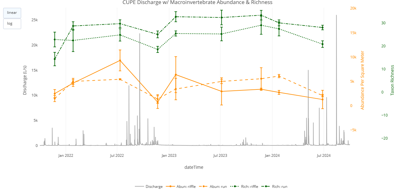
Snapshot of the interactive HTML plot generated in the code above using the `plotly` package. When running the code, the plot should be saved to your 'Documents' folder.
What kind of observations can be made when examining AIS discharge and AOS macroinvertebrate data on the same plotting field?
The standardized spatiotemporal design of NEON's aquatic data products allows one to easily run the same analysis for any NEON site. Given that all of NEON's 24 stream sites publish both AIS continuous discharge and AOS macroinvertebrate collection data products, users can substitute any 4-letter NEON stream site codes into this exercise to assess the relationship between stream discharge and macroinvertebrate abundance and richness.
Visit the Explore NEON Field Sites webpage to learn more about the different NEON aquatic sites. To run this exercise on a different combination of two sites, use find+replace to change the site IDs throughout the code.
Case Studies - Introduction
Now, we can take what we have learned about NEON AOS and AIS data and look at other case studies using different NEON data products. These case studies take you on a deeper dive into NEON data products and data wrangingling and visualization in R.
Case Study 1: Can relationships between sensor measurements and discrete water chemistry data be used to expand the temporal extent of ecologically-relevant analytes?
Before exploring this case study: This case study can be run independently of the introductory AOS and AIS data exploration code. This case study is coded to be run for 1 site. By default, we will focus on water years 2022-2024 at the West St. Louis Creek (WLOU) site, which is a high elevation stream in the Southern Rockies & Colorado Plateau Domain (D13). Set the following inputs prior to downloading data:
-
siteList <- c("WLOU") -
startWY <- 2022 -
endWY <- 2024
Learn more about the West St. Louis Creek site (D13-WLOU)
We are going to switch gears to a different kind of integration between AOS and AIS data. We evaluate the relationship between high-frequency fluorescent dissolved organic matter (fDOM) AIS data and dissolved organic carbon (DOC) data analyzed from AOS water chemistry grab samples to model a continuous DOC timeseries.
The data products downloaded here are:
AIS Data Products:
- Water quality (DP1.20288.001)
AOS Data Products:
- Chemical properties of surface water (DP1.20093.001)
First, download AOS data, run the duplicate check, and plot the data.
# download data of interest - AOS - Chemical properties of surface water

swc <- loadByProduct(dpID="DP1.20093.001",
                     site=siteList,
                     startdate=startWY_query,
                     enddate=endWY_query,
                     package="basic",
                     release= "current",
                     include.provisional=T,
                     token=Sys.getenv("NEON_TOKEN"),
                     check.size=F)

# unlist the variables and add to the global environment

list2env(swc, envir=.GlobalEnv)
The data table we are interested in here is swc_externalLabDataByAnalyte:
"Long-format results of chemical analysis of up to 28 unique analytes from
surface water and groundwater grab samples."
# check if there are duplicate DOC records

# what are the primary keys in swc_externalLabDataByAnalyte?

cat("Primary keys in swc_externalLabDataByAnalyte are:",
    paste(variables_20093$fieldName[
      variables_20093$table=="swc_externalLabDataByAnalyte"
      &variables_20093$primaryKey=="Y"
    ],
    collapse=", ")
    )
Primary keys in swc_externalLabDataByAnalyte are: sampleID, sampleCode, analyte
# identify duplicates in swc_externalLabDataByAnalyte

swc_externalLabDataByAnalyte_dups <- removeDups(swc_externalLabDataByAnalyte,
                                                variables_20093)

cat("There are",
    sum(swc_externalLabDataByAnalyte_dups$duplicateRecordQF%in%c(1, 2)),
    "duplicate records in 'swc_externalLabDataByAnalyte'")
There are 0 duplicate records in 'swc_externalLabDataByAnalyte'
Great, there are no duplicates!
Next, let's look at all the analytes returned for a single water sample. There can be up to 28 analytes returned per sample. The data is returned in 'long- format', meaning there is a row per analyte (up to 28 rows per sample) in lab data.
# show all the analytes published in the lab data

print(unique(swc_externalLabDataByAnalyte$analyte))

##  [1] "Ca"                     "Fe"                     "Cl"                     "K"                      "TPC"
##  [6] "TN"                     "Na"                     "F"                      "TPN"                    "SO4"
## [11] "NO3+NO2 - N"            "DIC"                    "Mn"                     "TDS"                    "Ortho - P"
## [16] "DOC"                    "NH4 - N"                "TDN"                    "TSS"                    "TP"
## [21] "UV Absorbance (254 nm)" "Si"                     "TOC"                    "TDP"                    "NO2 - N"
## [26] "Br"                     "UV Absorbance (280 nm)" "Mg"
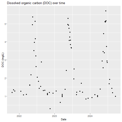
For this exercise, we will subset lab data to only dissolved organic carbon (DOC). Let's see what a DOC timeseries looks like.
# subset lab data to only dissolved organic carbon (DOC)

DOC <- swc_externalLabDataByAnalyte%>%
  filter(analyte=="DOC")

# plot a timeseries of DOC

DOC_plot <- DOC%>%
  ggplot(aes(x=collectDate, y=analyteConcentration))+
  geom_point()+
  labs(title="Dissolved organic carbon (DOC) over time",
       y="DOC (mg/L)",
       x="Date")

DOC_plot
Next, download AIS data, subset to the appropriate horizontalPosition, wrangle
the data for analysis, and plot the data.
# download data of interest - AIS - Water quality

waq <- loadByProduct(dpID="DP1.20288.001",
                     site=siteList,
                     startdate=startWY_query,
                     enddate=endWY_query,
                     package="basic",
                     release= "current",
                     include.provisional=T,
                     token=Sys.getenv("NEON_TOKEN"),
                     check.size=F)

# unlist the variables and add to the global environment

list2env(waq, envir=.GlobalEnv)
The data table we are interested in here is waq_instantaneous: "Wide-format
table published many water quality metrics in wide-format, including fDOM,
dissolved oxygen, specific conductance, pH, chlorophyll, and turbidity."
According to the NEON AIS spatial design, fDOM is only measured at the
downstream sensor set called S2. This corresponds to horizontal sensor positions
(HOR) that end in 2 (i.e., 102, 112, 132). At WLOU, the HOR we will subset to
is '102'. If you are runing this case study for another site, run
unique(waq_instantaneous$horizontalPosition) to identify the S2 HOR in the
data.
# subset to HOR 102 for WLOU

WAQ_S2 <- waq_instantaneous%>%
  filter(horizontalPosition==102)
Since this data product is not averaged, corrected, or gap-filled like the continuous discharge data we worked with earlier, there are two more important data wrangling steps to consider.
- Subset out any data with a 'final quality flag', which are indications of erroneous data in AIS data products.
- Average the data to a 15 minute interval to make the size of the data set easier to work with.
Let's do that prior to plotting.
# subset out QFs and average to 15 minute resolution

fDOM_15min <- WAQ_S2%>%
  filter(!is.na(rawCalibratedfDOM))%>%
  filter(fDOMFinalQF==0)%>%
  mutate(roundDate=round_date(endDateTime, "15 min"))%>%
  group_by(siteID, roundDate)%>%
  summarize(mean_fDOM=mean(rawCalibratedfDOM))
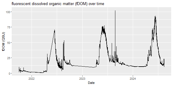
After wrangling, let's see what an fDOM timeseries looks like.
# plot a timeseries of fDOM

fDOM_plot <- fDOM_15min%>%
  ggplot(aes(x=roundDate, y=mean_fDOM))+
  geom_line()+
  labs(title="fluorescent dissolved organic matter (fDOM) over time",
       y="fDOM (QSU)",
       x="Date")

fDOM_plot
Both data products are published in Coordinated Universal Time (UTC), as are all AOS and AIS data, which makes joining across tables easy. Let's join the AOS and AIS data into a single data frame from which we will model the two variables.
# round DOC `collectDate` to the nearest 15 minute timestamp

DOC$roundDate <- round_date(DOC$collectDate, "15 min")

# perform a left-join, which will join an AIS DOC record to every AIS fDOM

# record based on matching timestamps

fDOM_DOC_join <- left_join(fDOM_15min, DOC, by="roundDate")
Create a linear regression to analyze the correlation of the two variables.
# use `lm` function to create a linear regression: DOC~fDOM

model <- lm(analyteConcentration~mean_fDOM, data=fDOM_DOC_join)

# view a summary of the regression model

print(summary(model))

##
## Call:
## lm(formula = analyteConcentration ~ mean_fDOM, data = fDOM_DOC_join)
##
## Residuals:
##      Min       1Q   Median       3Q      Max
## -0.69833 -0.24405 -0.00673  0.25586  0.67221
##
## Coefficients:
##             Estimate Std. Error t value Pr(>|t|)
## (Intercept) 0.781460   0.073660   10.61  1.3e-14 ***
## mean_fDOM   0.052742   0.001663   31.72  < 2e-16 ***
## ---
## Signif. codes:  0 '***' 0.001 '**' 0.01 '*' 0.05 '.' 0.1 ' ' 1
##
## Residual standard error: 0.334 on 52 degrees of freedom
##   (69854 observations deleted due to missingness)
## Multiple R-squared:  0.9509,	Adjusted R-squared:  0.9499
## F-statistic:  1006 on 1 and 52 DF,  p-value: < 2.2e-16
Visualize the regression with a fitted scatterplot.
# show a plot of the relationship with a linear trendline added

fDOM_DOC_plot <- fDOM_DOC_join%>%
  ggplot(aes(x=mean_fDOM, y=analyteConcentration))+
  geom_point()+
  geom_smooth(method="lm", se=T)+
  scale_x_continuous(limits=c(0, 60))+
  labs(title="AOS-DOC vs. AIS-fDOM",
       y="DOC (mg/L)",
       x="fDOM (QSU)")

fDOM_DOC_plot
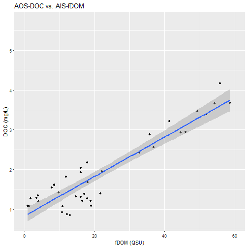
Given relatively high AIS data completeness and a correlative relationship between AOS-DOC and AIS-fDOM, Let's model DOC vs. fDOM from 2021-10-01 to 2024-09-30. We will add modeled continuous DOC as a column in the joined table.
# predict continuous doc based on the linear regression model coefficients

fDOM_DOC_join$fit <- predict(model,
                             newdata=fDOM_DOC_join,
                             interval="confidence")[, "fit"]

# add two more columns with predicted 95% CI uncertainty around the modeled DOC

conf_int <- predict(model, newdata=fDOM_DOC_join, interval="confidence")

fDOM_DOC_join$lwr <- conf_int[, "lwr"]

fDOM_DOC_join$upr <- conf_int[, "upr"]
With the modeled data added to our joined data table, let's plot the resulting
modeled DOC w/ uncertainty on the same plotting field as the DOC measured from
water chemistry grab samples. We will make this plot using plotly so we can
zoom in to see how well the AOS-DOC and modeled continuous DOC match up.
# create plot

fDOM_DOC_plot <- plot_ly(data=fDOM_DOC_join)%>%

  # plot uncertainty as a ribbon
  add_trace(x=~roundDate, y=~upr, name="95% CI",
            type='scatter', mode='line',
            line=list(color='lightgray'), legendgroup="95CI",
            showlegend=F)%>%
  add_trace(x=~roundDate, y=~lwr, name="95% CI",
            type='scatter', mode='none', fill='tonexty',
            fillcolor='lightgray', legendgroup="95CI")%>%

  # plot modeled DOC timeseries
  add_trace(x=~roundDate, y=~fit, name="Modeled DOC",
            type='scatter', mode='line',
            line=list(color='blue'))%>%

  # plot grab sample DOC
  add_trace(x=~roundDate, y=~analyteConcentration, name="Grab Sample DOC",
            type='scatter', mode='markers',
            marker=list(color='darkorange'))%>%

  # format title, axes, and legend
  layout(title="Dissolved Organic Carbon: Modelled & Grab Sample",
         xaxis=list(title="Date"),
         yaxis=list(title="DOC (mg/L)"),
         legend=list(xanchor='center',
                     yanchor='top',
                     orientation='h',
                     x=0.5, y=-0.2))


# save HTML plot to local documents folder

saveWidget(as_widget(fDOM_DOC_plot), paste0("~/", siteList, "_fDOM_DOC_model.html"))
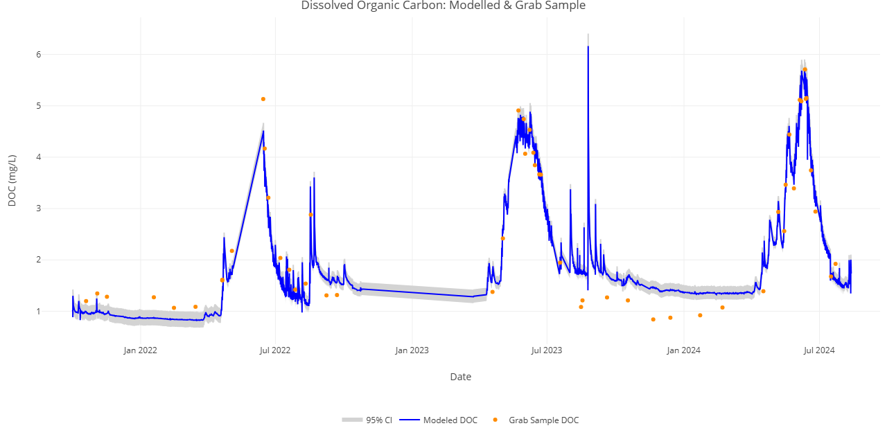
Snapshot of the interactive HTML plot generated in the code above using the `plotly` package. When running the code, the plot should be saved to your 'Documents' folder.
Discussion: This study shows the possibility of integrating AIS and AOS data to expand the temporal scale of estimated DOC in stream sites. At WLOU, estimated DOC matches well with grab sample DOC across mid- to high-range values, with uncertainty increasing at the low end of the timeseries. The relationship will continue to be expanded upon, following NEON’s flow-weighted sampling design.
The standardized nature of NEON data products and site designs allow for this and other analyses to be scaled across the observatory, revealing similarities and differences in the relationship across sites, and allowing for more detailed investigation of carbon dynamics in freshwater systems across the United States.
Try out this analysis at your favorite site! What environmental factors could contribute to the quality of this relationship at different NEON stream sites?
Case Study 2: Hurricane-impacted streams: Examine relationships between discharge, sediment particle size distribution, and macroinvertebrate abundance/diversity
Before exploring this case study: Run the introductory AOS and AIS data exploration code with the following variables set:
-
siteList <- c("CUPE","GUIL") -
startWY <- 2022 -
endWY <- 2024
In September 2022, Hurricane Fiona struck land in Puerto Rico as a Category 1 hurricane. Two NEON D04 aquatic sites were impacted. Here, we scale three data products across time to get an integrated look at how Hurricane Fiona (red line) affected the hydrology, morphology, and biology of two streams.
In this exercise, we will pull data from NEON Atlantic Neotropical Domain (D04). The aquatic sites in D04 are Rio Cupeyes (CUPE) and Rio Yahuecas (GUIL).
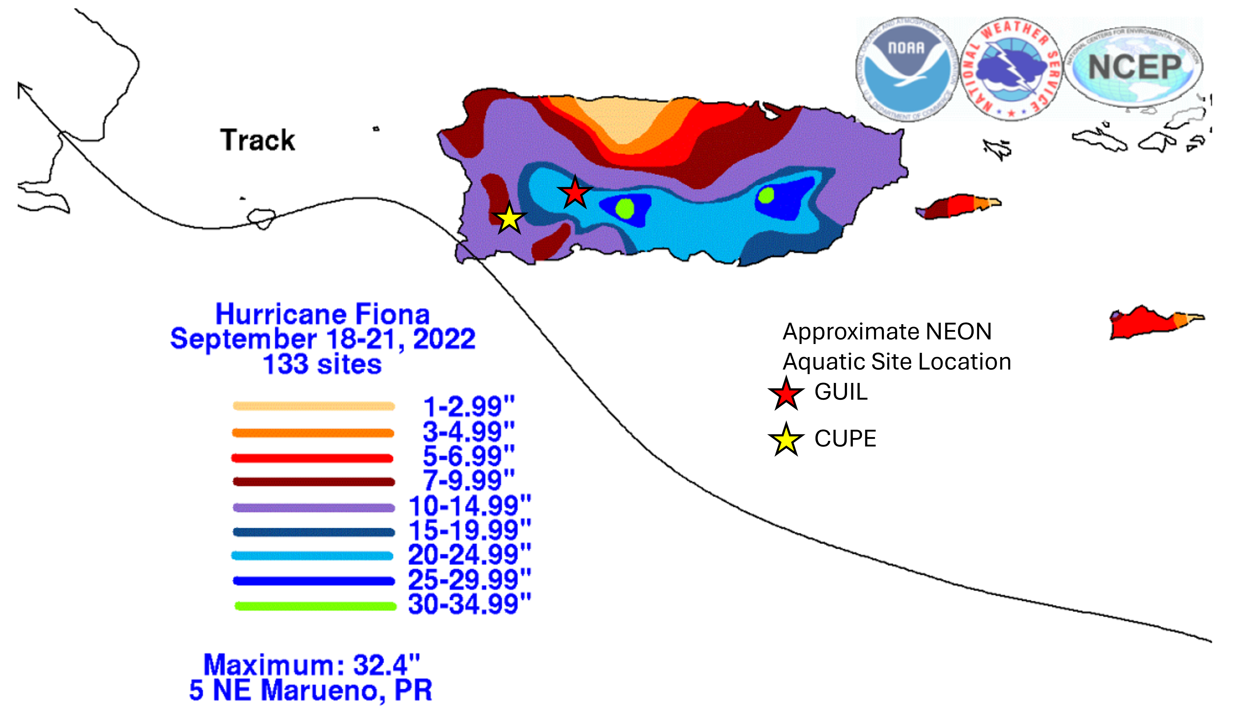
Total rainfall accumulation in Puerto Rico from Hurricane Fiona, overlaid with approximate locations of the two NEON D04 aquatic sites: CUPE, GUIL. Image source: https://www.nhc.noaa.gov/data/tcr/AL072022_Fiona.pdf
For this case study, we will look again at the relationship between stream discharge and macroinvertebrate abundance and richness with the hurricane event highlighted. We will compare the effects of the hurricane on stream hydrology and biology between the two sites.
We will also bring in a third NEON aquatic data product:
From the Stream morphology maps data product, we will examine the effect of Hurricane Fiona on streambed particle size distribution, expanding our exploration of NEON aquatic data to uncover linkages between the hydrology, morphology, and biology of NEON streams.
According to NOAA, Hurricane Fiona traveled through Puerto Rico between 18-21 September, 2022. Let's highlight that event in our combined AOS and AIS plots by adding a red vertical dashed line on 2022-09-19.
# identify the date of Fiona

fionaDate <- "2022-09-19"

# highlight Fiona at CUPE

AOS_AIS_plot_CUPE_Fiona <- AOS_AIS_plot_CUPE%>%
  # add dashed vertical line to plot created in previous exercise
  add_segments(x=as.POSIXct(fionaDate, tz="UTC"),
               xend=as.POSIXct(fionaDate, tz="UTC"),
               y=0,
               yend=max(csd_15_min$dischargeContinuous[
                 csd_15_min$siteID=="CUPE"],
                 na.rm=T),
               name="Fiona",
               line=list(color='red', dash='dash'))

# save HTML plot to local documents folder

saveWidget(as_widget(AOS_AIS_plot_CUPE_Fiona), "~/CUPE_INV_CSD_Fiona.html")

# highlight Fiona at GUIL

AOS_AIS_plot_GUIL_Fiona <- AOS_AIS_plot_GUIL%>%
  # add dashed vertical line to plot created in previous exercise
  add_segments(x=as.POSIXct(fionaDate, tz="UTC"),
               xend=as.POSIXct(fionaDate, tz="UTC"),
               y=0,
               yend=max(csd_15_min$dischargeContinuous[
                 csd_15_min$siteID=="GUIL"],
                 na.rm=T),
               name="Fiona",
               line=list(color='red', dash='dash'))

# save HTML plot to local documents folder

saveWidget(as_widget(AOS_AIS_plot_GUIL_Fiona), "~/GUIL_INV_CSD_Fiona.html")
Next, we will use the neonUtilities function loadByProduct() to load data
from the Stream morphology maps data product into R.
# download data of interest - AOS - Stream morphology maps

# the expanded download package is needed to read in the geo_pebbleCount table

geo <- loadByProduct(dpID="DP4.00131.001",
                     site=siteList,
                     startdate=startWY_query,
                     enddate=endWY_query,
                     package="expanded",
                     release= "current",
                     include.provisional=T,
                     token=Sys.getenv("NEON_TOKEN"),
                     check.size=F)

# unlist the variables and add to the global environment

list2env(geo, envir=.GlobalEnv)
There are many data tables included in this Level 4 AOS download package, but we are only interested in using one table for this exercise:
-
geo_pebbleCount- Sediment particle size data collected during pebble count sampling. Pebble count surveys are conducted once per year, typically during periods of baseflow at a given site.
Check for duplicates in geo_pebbleCount using removeDups().
# what are the primary keys in geo_pebbleCount?

cat("Primary keys in geo_pebbleCount are:",
    paste(variables_00131$fieldName[
      variables_00131$table=="geo_pebbleCount"
      &variables_00131$primaryKey=="Y"
    ],
    collapse=", ")
    )
Primary keys in geo_pebbleCount are: eventID, measurementLocation, pebbleCountNumber
# identify duplicates in geo_pebbleCount

geo_pebbleCount_dups <- removeDups(geo_pebbleCount,variables_00131)

cat("There are",
    sum(geo_pebbleCount_dups$duplicateRecordQF%in%c(1, 2)),
    "duplicate records in 'geo_pebbleCount'")
There are 0 duplicate records in 'geo_pebbleCount'
There are no duplicates! Let's proceed.
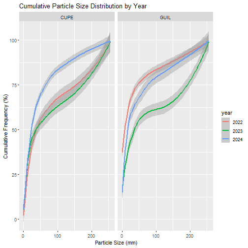
Next, let's wrangle the data and plot cumulative frequency curves to visualize particle size distributions for NEON D04 aquatic sites across water years 2022, 2023, and 2024.
The pebbleSize field in geo_pebbleCount is published as a categorical
variable reporting the range of the particle size (e.g., '4 - 5.6 mm: fine
gravel'). For plotting purposes, we will convert the categorical variable to
numeric by singling out the lower number of the categorical size range.
# convert pebbleSize to numeric

geo_pebbleCount$pebbleSize_num <- NA

geo_pebbleCount$pebbleSize_num[
  geo_pebbleCount$pebbleSize=="< 2 mm: silt/clay"
  ] <- 0

geo_pebbleCount$pebbleSize_num[
  geo_pebbleCount$pebbleSize=="< 2 mm: sand"
  ] <- 0

geo_pebbleCount$pebbleSize_num[
  geo_pebbleCount$pebbleSize=="2 - 2.8 mm: very coarse sand"
  ] <- 2

geo_pebbleCount$pebbleSize_num[
  geo_pebbleCount$pebbleSize=="2.8 - 4 mm: very fine gravel"
  ] <-2.8

geo_pebbleCount$pebbleSize_num[
  geo_pebbleCount$pebbleSize=="4 - 5.6 mm: fine gravel"
  ] <- 4

geo_pebbleCount$pebbleSize_num[
  geo_pebbleCount$pebbleSize=="5.6 - 8 mm: fine gravel"
  ] <- 5.6

geo_pebbleCount$pebbleSize_num[
  geo_pebbleCount$pebbleSize=="8 - 11 mm: medium gravel"
  ] <- 8

geo_pebbleCount$pebbleSize_num[
  geo_pebbleCount$pebbleSize=="11 - 16 mm: medium gravel"
  ] <- 11

geo_pebbleCount$pebbleSize_num[
  geo_pebbleCount$pebbleSize=="16 - 22.6 mm: coarse gravel"
  ] <- 16

geo_pebbleCount$pebbleSize_num[
  geo_pebbleCount$pebbleSize=="22.6 - 32 mm: coarse gravel"
  ] <- 22.6

geo_pebbleCount$pebbleSize_num[
  geo_pebbleCount$pebbleSize=="32 - 45 mm: very coarse gravel"
  ] <- 32

geo_pebbleCount$pebbleSize_num[
  geo_pebbleCount$pebbleSize=="45 - 64 mm: very coarse gravel"
  ] <- 45

geo_pebbleCount$pebbleSize_num[
  geo_pebbleCount$pebbleSize=="64 - 90 mm: small cobble"
  ] <- 64

geo_pebbleCount$pebbleSize_num[
  geo_pebbleCount$pebbleSize=="90 - 128 mm: medium cobble"
  ] <- 90

geo_pebbleCount$pebbleSize_num[
  geo_pebbleCount$pebbleSize=="128 - 180 mm: large cobble"
  ] <- 128

geo_pebbleCount$pebbleSize_num[
  geo_pebbleCount$pebbleSize=="180 - 256 mm: large cobble"
  ] <- 180

geo_pebbleCount$pebbleSize_num[
  geo_pebbleCount$pebbleSize=="> 256 mm: boulder"
  ] <- 256

geo_pebbleCount$pebbleSize_num[
  geo_pebbleCount$pebbleSize=="> 256 mm: bedrock"
  ] <- 256
Next, calculate a cumulative sum of frequency across particle size, and group by site and year for plotting.
# group by 'siteID' and 'surveyEndDate'` and calculate frequency

geo_pebbleCount_freq <- geo_pebbleCount%>%
  group_by(siteID, surveyEndDate, eventID, pebbleSize_num)%>%
  summarise(frequency=n()/200)

# calculate a cumulative sum of frequency per event ID

for(e in 1:length(unique(geo_pebbleCount_freq$eventID))){
  eventID_freq <- geo_pebbleCount_freq%>%
    filter(eventID==unique(geo_pebbleCount$eventID)[e])
  eventID_freq$CumulativeFreq <- cumsum(eventID_freq$frequency)*100
  if(e==1){
    geo_pebbleCount_freqCumm <- eventID_freq
  }else{
    geo_pebbleCount_freqCumm <- rbind(geo_pebbleCount_freqCumm, eventID_freq)
  }
}

# assign a year to each survey

geo_pebbleCount_freqCumm <- geo_pebbleCount_freqCumm%>%
  mutate(year=format(surveyEndDate, "%Y"))
Now, plot cumulative particle size distributions across sites and years.
# create cumulative frequency curve plot using `geom_smooth`

geo_pebbleCount_freqCumm%>%
  ggplot(aes(x=pebbleSize_num, y=CumulativeFreq, color=year)) +
  geom_smooth(method="loess", se=T, linewidth=0.75) +
  labs(title="Cumulative Particle Size Distribution by Year",
       x="Particle Size (mm)", y="Cumulative Frequency (%)") +
  facet_wrap(~siteID)
To effectively view the particle size distribution data with the other two data
products, we will embed them as ggplot subplots in the larger plotly plot.
# generate small, simple subplots of each pebble count survey

# loop through each site and year to make plot and save to the working directory

for(s in 1:length(unique(geo_pebbleCount_freqCumm$siteID))){
  currSite <- unique(geo_pebbleCount_freqCumm$siteID)[s]
  for(y in 1:length(unique(geo_pebbleCount_freqCumm$year))){
    currYear <- unique(geo_pebbleCount_freqCumm$year)[y]
    currPlot <- geo_pebbleCount_freqCumm%>%
      filter(siteID==currSite
                    &year==currYear)%>%
      ggplot(aes(x=pebbleSize_num, y=CumulativeFreq)) +
      geom_smooth(method="loess", se=T, linewidth=0.75) +
      labs(x=NULL, y=NULL)+
      scale_y_continuous(limits=c(0, 105))+
      scale_x_continuous(limits=c(0, 260))+
      theme_bw()+
      theme(text=element_text(size=18))
    ggsave(plot=currPlot,
                    filename=paste0("~/images/psd_", currSite, currYear, ".png"),
                    width=4, height=7, units="cm")
  }
}

# re-generate the CUPE plot with particle size distribution subplots added

AOS_AIS_plot_CUPE_Fiona <- AOS_AIS_plot_CUPE_Fiona%>%
  layout(images=list(

    # show the CUPE 2022 pebble count survey, conducted 2022-04
    list(source=dataURI(file="~/images/psd_CUPE2022.png"),
         x=0.05, y=0.7,
         sizex=0.25, sizey=0.25,
         xref="paper", yref="paper",
         xanchor="left", yanchor="bottom"),

    # show the CUPE 2023 pebble count survey, conducted 2022-05
    list(source=dataURI(file="~/images/psd_CUPE2023.png"),
         x=0.4, y=0.7,
         sizex=0.25, sizey=0.25,
         xref="paper", yref="paper",
         xanchor="left", yanchor="bottom"),

    # show the CUPE 2024 pebble count survey, conducted 2022-05
    list(source=dataURI(file="~/images/psd_CUPE2024.png"),
         x=0.7, y=0.7,
         sizex=0.25, sizey=0.25,
         xref="paper", yref="paper",
         xanchor="left", yanchor="bottom")

    ))

# save HTML plot to local documents folder

saveWidget(as_widget(AOS_AIS_plot_CUPE_Fiona), "~/CUPE_INV_CSD_GEO_Fiona.html")

# re-generate the GUIL plot with particle size distribution subplots added

AOS_AIS_plot_GUIL_Fiona <- AOS_AIS_plot_GUIL_Fiona%>%
  layout(images=list(

    # show the GUIL 2022 pebble count survey, conducted 2022-04
      list(source=dataURI(file="~/images/psd_GUIL2022.png"),
         x=0.05, y=0.7,
         sizex=0.25, sizey=0.25,
         xref="paper", yref="paper",
         xanchor="left", yanchor="bottom"),

    # show the GUIL 2023 pebble count survey, conducted 2023-03
    list(source=dataURI(file="~/images/psd_GUIL2023.png"),
         x=0.35, y=0.7,
         sizex=0.25, sizey=0.25,
         xref="paper", yref="paper",
         xanchor="left", yanchor="bottom"),

    # show the GUIL 2024 pebble count survey, conducted 2024-07
    list(source=dataURI(file="~/images/psd_GUIL2024.png"),
         x=0.75, y=0.7,
         sizex=0.25, sizey=0.25,
         xref="paper", yref="paper",
         xanchor="left", yanchor="bottom")

    ))

# save HTML plot to local documents folder

saveWidget(as_widget(AOS_AIS_plot_GUIL_Fiona), "~/_INV_CSD_GEO_Fiona.html")
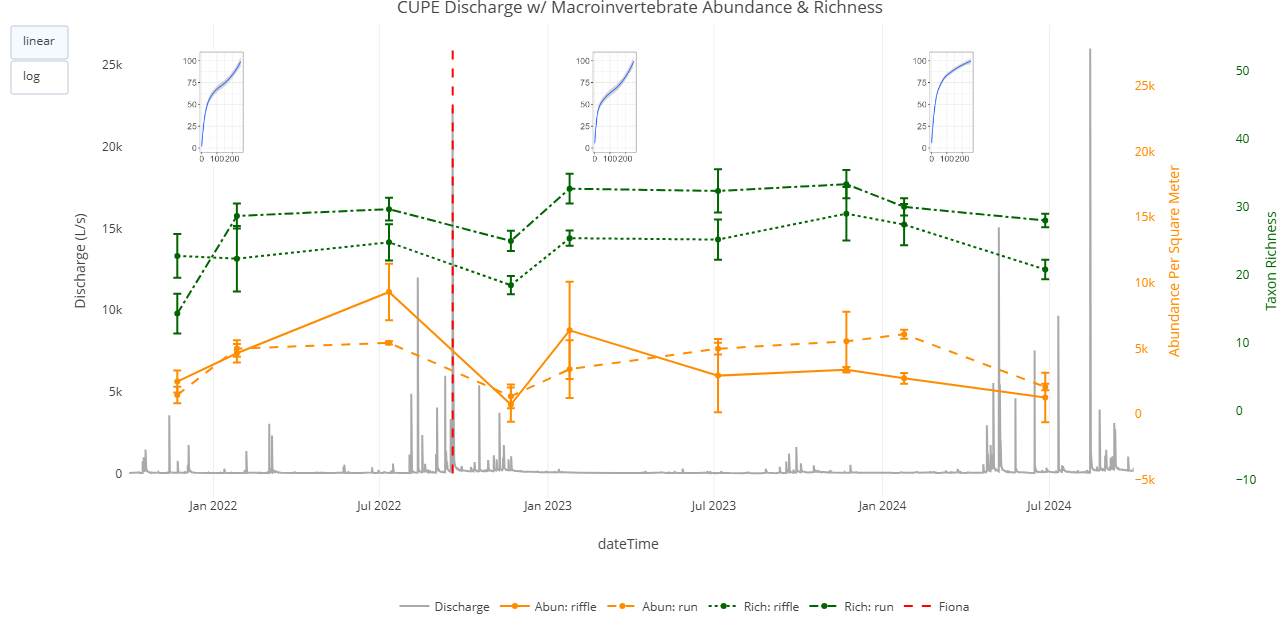
Snapshot of the interactive HTML plot generated in the code above using the `plotly` package. When running the code, the plot should be saved to your 'Documents' folder.
Discussion: With the three data products viewed together in relation to the Hurricane Fiona event, there are several observations that can be made:
-
Hydrology
- Both sites were hit with heavy rain, with CUPE discharge reaching nearly 20,000 L/s at its peak.
- Sensor infrastructure at GUIL was temporarily compromised during the storm, resulting in a data gap.
-
Morphology
- The sediment particle size distribution data suggests that CUPE sediment remained relatively stable pre- and post-storm, while GUIL showed heavier loss of small sediment via scouring.
-
Biology
- While both sites show a large decrease in macroinvertebrate abundance post-storm, GUIL shows a more negative effect to macroinvertebrate diversity relative to CUPE.
- Both sites show a trend back to pre-storm abundance and diversity numbers by the following spring bout.
By integrating data products across time, we observe disparate effects of Hurricane Fiona on NEON D04 sites, with a potential relationship being revealed between the stability of the streambed substrate and the loss of macroinvertebrate diversity immediately following a major precipitation event.
Case Study 3: Macroinvertebrates in drying streams: visualize the interplay between abundance, richness, and flow within and across water years
Before exploring this case study: Run the introductory AOS and AIS data exploration code with the following variables set:
-
siteList <- c("KING","ARIK","SYCA) -
startWY <- 2022 -
endWY <- 2025
Here, we highlight three NEON non-perennial stream sites that undergo partial-to-complete drying on an annual basis, bringing stream discharge to zero (0) at some point in each water year.
Kings Creek, Prairie Peninsula Domain, Kansas (KING, D06, KS):
Learn more about the Kings Creek site (D06-KING)

PhenoCam images comparing peak flow (left) and dry conditions (right) for KING in water year 2024.
Arikaree River, Central Plains Domain, Colorado (ARIK, D10, CO):
Learn more about the Arikaree River site (D10-ARIK)
PhenoCam images comparing peak flow (left) and dry conditions (right) for ARIK in water year 2024.
Sycamore Creek, Desert Southwest Domain, Arizona (SYCA, D14, AZ):
Learn more about the Sycamore Creek site (D14-SYCA)
PhenoCam images comparing peak flow (left) and dry conditions (right) for SYCA in water year 2024.
In these non-perennial streams, understanding when flow arrives, how quickly it accumulates, and how benthic macroinvertebrate communities respond is critical for predicting the ecological consequences of changing precipitation patterns and drought frequency.
We will use advanced plotting techniques in R to plot benthic macroinvertebrate
abundance and richness over a cumulative discharge curve per water year. We will
then stack water years vertically for a site. We will use a combination of the
plotly, htmltools, and htmlwidgets packages in R to create interactive and
linked stacked plots. Using a cumulative discharge curve will allow you to
easily identify the onset, magnitude, duration, and cessation of flow, and
assess the effect those hydrologic parameters have on macroinvertebrate
communities within and across water years at a site.
First, let's wrangle the discharge and macroinvertebrate data to 1) assign every record a water year, and 2) calculate cumulative flow across each water year.
# assign each discharge record a water year

csd_15_min <- csd_15_min%>%
  mutate(waterYear=ifelse(month(startDateTime)>=10,
                          year(startDateTime)+1,
                          year(startDateTime)),
         waterYearStart=as.Date(paste0(waterYear-1, "-10-01")),
         dayOfWaterYear=as.integer(as.Date(startDateTime)-waterYearStart)+1,
         plotDateWY=as.Date("1999-10-01") + (dayOfWaterYear-1))

# group by site ID and water year and summarize a cumulative sum of discharge to make a cumulative flow curve

csd_15_min_summ <- csd_15_min%>%
  arrange(siteID, waterYear, startDateTime)%>%
  group_by(siteID, waterYear)%>%
  mutate(cumulativeFlow=cumsum(dischargeContinuous),
         cumulativeFlowPct=100*cumulativeFlow/max(cumulativeFlow, na.rm=TRUE))%>%
  ungroup()

# assign water year and day-of-water-year to invert abundance summary

inv_abundance_case2 <- inv_abundance_summ%>%
  ungroup()%>%
  mutate(waterYear=ifelse(month(collectDate)>=10,
                          year(collectDate)+1,
                          year(collectDate)),
         waterYearStart=as.Date(paste0(waterYear-1, "-10-01")),
         dayOfWaterYear=as.integer(as.Date(collectDate)-waterYearStart)+1,
         plotDateWY=as.Date("1999-10-01") + (dayOfWaterYear-1),
         abun_M2_sum_se=coalesce(abun_M2_sum_se, 0))%>%
  arrange(siteID, waterYear, habitatType, dayOfWaterYear)

# assign water year and day-of-water-year to invert richness summary

inv_richness_case2 <- inv_diversity_summ%>%
  filter(indexName=="richness")%>%
  ungroup()%>%
  mutate(waterYear=ifelse(month(collectDate)>=10,
                          year(collectDate)+1,
                          year(collectDate)),
         waterYearStart=as.Date(paste0(waterYear-1, "-10-01")),
         dayOfWaterYear=as.integer(as.Date(collectDate)-waterYearStart)+1,
         plotDateWY=as.Date("1999-10-01") + (dayOfWaterYear-1),
         se=coalesce(se, 0))%>%
  arrange(siteID, waterYear, habitatType, dayOfWaterYear)
Now, we will create our visuals. For each site, we will create a plot that shows the following:
- Cumulative flow curve for each water year
- Benthic Macroinvertebrate abundance (y-axis 2) and richness (y-axis 3) by habitat type
- Each water year plot stacked in a single column
- Axes ranges and limits set identically in all stacked plots
- Traces linked in a single legend at top of stacked plots
Once the plots are generated and saved to your local machine, we can view trends and relationships across space and time.
# build one stacked plot per site with cumulative flow, abundance, and richness

for(s in 1:length(siteList)){
  waterYears <- sort(
    unique(csd_15_min_summ$waterYear[csd_15_min_summ$siteID==siteList[s]]))
  # set fixed axis ranges for this site so all WY panels are directly comparable
  site_flow <- csd_15_min_summ%>%
    filter(siteID==siteList[s])
  site_abun <- inv_abundance_case2%>%
    filter(siteID==siteList[s])
  site_rich <- inv_richness_case2%>%
    filter(siteID==siteList[s])
  abun_labels <- sort(unique(paste0("Abun: ", site_abun$habitatType)))
  rich_labels <- sort(unique(paste0("Rich: ", site_rich$habitatType)))
  x_range <- range(site_flow$plotDateWY, na.rm=TRUE)
  y1_range <- c(0, max(site_flow$cumulativeFlow, na.rm=TRUE))
  abun_upper <- c(site_abun$abun_M2_sum_mean + site_abun$abun_M2_sum_se,
                  site_abun$abun_M2_sum_mean)
  if(all(is.na(abun_upper))){
    y2_range <- c(0, 1)
  }else{
    y2_range <- c(0, max(abun_upper, na.rm=TRUE))
  }
  rich_upper <- c(site_rich$mean + site_rich$se,
                  site_rich$mean)
  if(all(is.na(rich_upper))){
    y3_range <- c(0, 1)
  }else{
    y3_range <- c(0, max(rich_upper, na.rm=TRUE))
  }
  # create each subplot and store in list
  wyPlots <- list()
  for(wy in 1:length(waterYears)){
    # subset down to current site and water year
    cumsumPlot <- plot_ly(data=csd_15_min_summ%>%
                            filter(siteID==siteList[s]
                                   &waterYear==waterYears[wy]))%>%

      # cumulative flow curve
      add_trace(x=~plotDateWY,
                y=~cumulativeFlow,
                type="scatter",
                mode="lines",
                line=list(color="darkgray"),
                name="Cumulative Flow",
                showlegend=F)%>%

      # benthic macroinvertebrate abundance by habitat type
      add_trace(data=inv_abundance_case2%>%
                  filter(siteID==siteList[s]
                                &waterYear==waterYears[wy]),
                x=~plotDateWY,
                y=~abun_M2_sum_mean,
                split=~paste0("Abun: ", habitatType),
                linetype=~paste0("Abun: ", habitatType),
                yaxis="y2",
                type="scatter",
                mode="lines+markers",
                error_y=~list(array=abun_M2_sum_se,
                              color='darkorange',
                              visible=TRUE),
                marker=list(color="darkorange"),
                line=list(color="darkorange", width=2),
                showlegend=F)%>%

      # benthic macroinvertebrate richness by habitat type
      add_trace(data=inv_richness_case2%>%
                  filter(siteID==siteList[s]
                                &waterYear==waterYears[wy]),
                x=~plotDateWY,
                y=~mean,
                split=~paste0("Rich: ", habitatType),
                linetype=~paste0("Rich: ", habitatType),
                yaxis="y3",
                type="scatter",
                mode="lines+markers",
                error_y=~list(array=se,
                              color='darkgreen',
                              visible=TRUE),
                marker=list(color="darkgreen"),
                line=list(color="darkgreen", width=2),
                showlegend=F)%>%

      # plot layout
      layout(
        title=paste0(siteList[s], " | WY ", waterYears[wy]),
        xaxis=list(title="Month-Day",
                   automargin=TRUE,
                   domain=c(0, 0.9),
             range=x_range,
             type="date",
             tick0="1999-10-01",
             dtick="M1",
             tickformat="%m-%d"),
        yaxis=list(
          side='left',
          title='Cumulative Flow (L/s)',
          showgrid=FALSE,
          zeroline=FALSE,
          automargin=TRUE,
          range=y1_range),
        yaxis2=list(
          side='right',
          overlaying="y",
          title='Abundance Per Square Meter',
          showgrid=FALSE,
          automargin=TRUE,
          zeroline=FALSE,
          range=y2_range,
          tickfont=list(color='darkorange'),
          titlefont=list(color='darkorange')),
        yaxis3=list(
          side='right',
          overlaying="y",
          anchor="free",
          title='Taxon Richness',
          showgrid=FALSE,
          zeroline=FALSE,
          automargin=TRUE,
          range=y3_range,
          tickfont=list(color='darkgreen'),
          titlefont=list(color='darkgreen'),
          position=0.99)
      )

    wyPlots[[wy]] <- cumsumPlot
  }
  # Create custom legend
  legend_items <- c(
    list(tags$button(
      type="button",
      class="case2-legend-item active",
      `data-trace-name`="Cumulative Flow",
      HTML("<span style='display:inline-block;width:18px;border-top:3px solid darkgray;margin-right:6px;vertical-align:middle;'></span>Cumulative Flow")
    )),
    lapply(abun_labels, function(lbl) {
      tags$button(
        type="button",
        class="case2-legend-item active",
        `data-trace-name`=lbl,
        HTML(paste0("<span style='display:inline-block;width:18px;border-top:3px solid darkorange;margin-right:6px;vertical-align:middle;'></span>", lbl))
      )
    }),
    lapply(rich_labels, function(lbl) {
      tags$button(
        type="button",
        class="case2-legend-item active",
        `data-trace-name`=lbl,
        HTML(paste0("<span style='display:inline-block;width:18px;border-top:3px solid darkgreen;margin-right:6px;vertical-align:middle;'></span>", lbl))
      )
    })
  )
  legendSyncJs <- sprintf(
    paste(
      "(function(){",
      "  var container=document.getElementById('case2_%s');",
      "  if (!container || container.dataset.legendBound === '1') return;",
      "  container.dataset.legendBound='1';",
      "  container.addEventListener('click', function(ev){",
      "    var btn=ev.target.closest('.case2-legend-item');",
      "    if (!btn) return;",
      "    var traceName=btn.getAttribute('data-trace-name');",
      "    var hideTrace=!btn.classList.contains('inactive');",
      "    var newVis=hideTrace ? false : true;",
      "    var plots=container.querySelectorAll('.js-plotly-plot');",
      "    plots.forEach(function(gd){",
      "      var idx=[];",
      "      for (var i=0; i < gd.data.length; i++) {",
      "        if (gd.data[i].name === traceName) idx.push(i);",
      "      }",
      "      if (idx.length) Plotly.restyle(gd, {visible: newVis}, idx);",
      "    });",
      "    btn.classList.toggle('inactive');",
      "  });",
      "})();",
      sep="\n"
    ),
    siteList[s]
  )
  # build final stacked plots
  curr_plot <- tagList(
    tags$h3(
      paste0("Cumulative Flow, Abundance, and Richness for ",
             siteList[s], " (Stacked by Water Year)")
    ),
    div(
      id=paste0("case2_", siteList[s]),
      tags$div(
        style=paste(
          "display:flex;flex-wrap:wrap;gap:8px;align-items:center;",
          "padding:8px 10px;margin:0 0 8px 0;background:#ffffff;",
          "border:1px solid #d9d9d9;border-radius:4px;"
        ),
        legend_items
      ),
      tags$style(HTML(
        ".case2-legend-item {background:#fff;border:1px solid #cfcfcf;border-radius:4px;padding:4px 8px;cursor:pointer;font-size:12px;}\n.case2-legend-item.inactive {opacity:0.45;}"
      )),
      wyPlots
    ),
    tags$script(HTML(legendSyncJs))
  )

  # save HTML plot to local documents folder
  output_file <- file.path(path.expand("~"), paste0(siteList[s], "_cumSumWY.html"))
  save_html(
    browsable(curr_plot),
    file=output_file,
    libdir=paste0(siteList[s], "_cumSumWY_files")
  )
}
Discussion: These visualization tools allow us to examine the interplay between discharge and macroinvertebrates across space and time. For example, on the scale of an individual sampling event (bout), you can observe the types of habitats sampled, the macroinvertebrate abundance and diversity in each habitat type, and the magnitude and slope of the cumulative flow at that point in the year.
Expanding our temporal scope, we want make observations across a single water year of macroinvertebrate bouts and discharge, such as:
- KING:
- WY 2022 - Shows high abundance and diversity in the spring bout before flow returns to the stream. The data is all from pool habitats, in which we see a steep decline in abundance and richness when water returns in the summertime.
- WY 2025 - virtually all of the year's flow came from a single event. This allowed for summer invert sampling to take place in both pool and riffle habitats. By the time of the fall bout, sampling was, once again, constrained to only pools.
- SYCA
- 2022 - Shows a massive spike in run abundance as the stream looks to be slowing in flow accumulation for the water year.
- 2025 - Complete dryness for an entire water year. All invert sampling was impractical.
The highlight of these visual tools is to show how NEON's standardized observational and instrumented monitoring allows you to gain unique insight into trends and relationships across large spatial and temporal scales. Let's see what we can observe about the trends and relationships between flow and benthic macroinvertebrates in NEON's non-perennial streams across space (multiple sites) and time (multiple water years).
- KING across time:
- Across the four water years observed, we see that KING alternated between water years with relatively high cumulative flow (2022, 2024) and water years with relatively low cumulative flow (2023, 2025).
- Spring sampling was impractical in 2023, 2024, and 2025 from lack of habitats due to drying.
- When water is returning and flowing through the stream, there is similar abundance in both pools and riffles, but riffle richness is consistently higher relative to pool richness across water years.
- ARIK across time:
- Overall water availability is much lower in 2022 than the subsequent years.
- Across all the summer bouts, pool habitats are the most common habitat sampled. Trends in the relationship between macroinvertebrate matrices and cumulative flow are visible, with pool abundance being negatively correlated with the magnitude of cumulative flow in a water year, and pool richness being positively correlated.
- During the spring bout each water year, there are the same trends in richness and abundance: pool abundance is higher than run abundance; pool richness is lower than run richness; abundance values by habitat type are much closer than richness values by habitat type.
- SYCA across time:
- Run abundance is consistently either comparable or less than riffle abundance, with the glaring exception of the 'summer' bout of 2022. There is much less water availability in 2022 relative to 2023 and 2024, which could explain the differences.
- Trends in richness are present across all water years, with riffle richness consistently higher than run richness, and peaks in richness during the 'summer' bouts, with 'spring' and 'fall' richness being lower.
- All streams across space:
- Across sites, there looks to be a similar trend in abundance where, before flowing water returns to the stream, abundance is high. Once water returns, abundance crashes, then recovers to varying degrees as flow persists.
- At ARIK and KING, we are more likely to see spring or fall bouts conducted during periods of partial dryness, where pool habitats are common. At SYCA, flow returns and ceases more quickly, making it less likely that sampling will take place during periods of partial dryness. This leads to interesting differences when looking at the sites, as ARIK and KING reveal more about the transition from dry-flow, whereas SYCA reveals more about the transition from flow-dry.