Workshop
NEON Brownbag: Working With Hyperspectral Imagery in HDF5 Format in R
NEON
This workshop will providing hands on experience with working with hyperspectral imagery in hierarchical data formats (HDF5) in R. It will also cover basic raster data analysis in R.
- Explain what hyperspectral remote sensing data are.
- Create and read from HDF5 files containing spatial data in R.
- Describe the key attributes of raster data that you need to spatially locate raster data in R.
Things to do before the workshop
To participant in this workshop, you will need a laptop with the most current version of R and, preferably, RStudio loaded on your computer. For details on setting up R & RStudio in Mac, PC, or Linux operating systems please see Additional Set up Resources below
R Libraries to Install
Please have these packages installed and updated prior to the start of the workshop.
-
rhdf5:
source("http://bioconductor.org/biocLite.R"); biocLite("rhdf5") -
raster:
install.packages("raster") -
rgdal:
install.packages("rgdal")
Updating R Packages
In RStudio, you can go to Tools --> Check for package updates to update previously installed packages on your computer.
Or you can use update.packages() to update all packages that are installed in R automatically.
More on Packages in R
Data to Download
[[nid:6330]]
Background Materials
Schedule
The workshop is held in the classroom that the NEON headquarters in Boulder, CO.
Additional Set Up Instructions
R & RStudio
Prior to the workshop you should have R and, preferably, RStudio installed on your computer.
[[nid:6408]] [[nid:6512]]
Install HDFView
The free HDFView application allows you to explore the contents of an HDF5 file.
To install HDFView:
-
Click to go to the download page.
-
From the section titled HDF-Java 2.1x Pre-Built Binary Distributions select the HDFView download option that matches the operating system and computer setup (32 bit vs 64 bit) that you have. The download will start automatically.
-
Open the downloaded file.
- Mac - You may want to add the HDFView application to your Applications directory.
- Windows - Unzip the file, open the folder, run the .exe file, and follow directions to complete installation.
- Open HDFView to ensure that the program installed correctly.
QGIS (Optional)
QGIS is a cross-platform Open Source Geographic Information system.
Online LiDAR Data/las Viewer (Optional)
Plas.io is a open source LiDAR data viewer developed by Martin Isenberg of Las Tools and several of his colleagues.
An Introduction to Remote Sensing
Please watch this video on remote sensing prior to the workshop
Image Raster Data in R - An Intro
This tutorial will walk you through the fundamental principles of working with image raster data in R.
Learning Objectives
After completing this activity, you will be able to:
- Import multiple image rasters and create a stack of rasters.
- Plot three band RGB images in R.
- Export single band and multiple band image rasters in R.
Things You’ll Need To Complete This Tutorial
You will need the most current version of R and, preferably, RStudio loaded
on your computer to complete this tutorial.
Install R Packages
-
raster:
install.packages("raster") -
rgdal:
install.packages("rgdal") -
sp:
install.packages("sp")
More on Packages in R – Adapted from Software Carpentry.
Download Data
NEON Teaching Data Subset: Field Site Spatial Data
These remote sensing data files provide information on the vegetation at the National Ecological Observatory Network's San Joaquin Experimental Range and Soaproot Saddle field sites. The entire dataset can be accessed by request from the NEON Data Portal.
Download DatasetThis data download contains several files. You will only need the RGB .tif files for this tutorial. The path to this file is: NEON-DS-Field-Site-Spatial-Data/SJER/RGB/* . The other data files in the downloaded data directory are used for related tutorials. You should set your working directory to the parent directory of the downloaded data to follow the code exactly.
Recommended Reading
You may benefit from reviewing these related resources prior to this tutorial:
Raster Data
Raster or "gridded" data are data that are saved in pixels. In the spatial world, each pixel represents an area on the Earth's surface. An color image raster is a bit different from other rasters in that it has multiple bands. Each band represents reflectance values for a particular color or spectra of light. If the image is RGB, then the bands are in the red, green and blue portions of the electromagnetic spectrum. These colors together create what we know as a full color image.

Work with Multiple Rasters
In
a previous tutorial,
we loaded a single raster into R. We made sure we knew the CRS
(coordinate reference system) and extent of the dataset among other key metadata
attributes. This raster was a Digital Elevation Model so there was only a single
raster that represented the ground elevation in each pixel. When we work with
color images, there are multiple rasters to represent each band. Here we'll learn
to work with multiple rasters together.
Raster Stacks
A raster stack is a collection of raster layers. Each raster layer in the raster stack needs to have the same
- projection (CRS),
- spatial extent and
- resolution.
You might use raster stacks for different reasons. For instance, you might want to group a time series of rasters representing precipitation or temperature into one R object. Or, you might want to create a color images from red, green and blue band derived rasters.
In this tutorial, we will stack three bands from a multi-band image together to create a composite RGB image.
First let's load the R packages that we need: sp and raster.
# load the raster, sp, and rgdal packages
library(raster)
library(sp)
library(rgdal)

# set the working directory to the data
#setwd("pathToDirHere")
wd <- ("~/Git/data/")
setwd(wd)
Next, let's create a raster stack with bands representing
- blue: band 19, 473.8nm
- green: band 34, 548.9nm
- red; band 58, 669.1nm
This can be done by individually assigning each file path as an object.
# import tiffs
band19 <- paste0(wd, "NEON-DS-Field-Site-Spatial-Data/SJER/RGB/band19.tif")
band34 <- paste0(wd, "NEON-DS-Field-Site-Spatial-Data/SJER/RGB/band34.tif")
band58 <- paste0(wd, "NEON-DS-Field-Site-Spatial-Data/SJER/RGB/band58.tif")

# View their attributes to check that they loaded correctly:
band19

## [1] "~/Git/data/NEON-DS-Field-Site-Spatial-Data/SJER/RGB/band19.tif"

band34

## [1] "~/Git/data/NEON-DS-Field-Site-Spatial-Data/SJER/RGB/band34.tif"

band58

## [1] "~/Git/data/NEON-DS-Field-Site-Spatial-Data/SJER/RGB/band58.tif"
Note that if we wanted to create a stack from all the files in a directory (folder)
you can easily do this with the list.files() function. We would use
full.names=TRUE to ensure that R will store the directory path in our list of
rasters.
# create list of files to make raster stack
rasterlist1 <- list.files(paste0(wd,"NEON-DS-Field-Site-Spatial-Data/SJER/RGB", full.names=TRUE))

rasterlist1

## character(0)
Or, if your directory consists of some .tif files and other file types you don't want in your stack, you can ask R to only list those files with a .tif extension.
rasterlist2 <-  list.files(paste0(wd,"NEON-DS-Field-Site-Spatial-Data/SJER/RGB", full.names=TRUE, pattern="tif"))

rasterlist2

## character(0)
Back to creating our raster stack with three bands. We only want three of the
bands in the RGB directory and not the fourth band90, so will create the stack
from the bands we loaded individually. We do this with the stack() function.
# create raster stack
rgbRaster <- stack(band19,band34,band58)

# example syntax for stack from a list
#rstack1 <- stack(rasterlist1)
This has now created a stack that is three rasters thick. Let's view them.
# check attributes
rgbRaster
## class : RasterStack
## dimensions : 502, 477, 239454, 3 (nrow, ncol, ncell, nlayers)
## resolution : 1, 1 (x, y)
## extent : 256521, 256998, 4112069, 4112571 (xmin, xmax, ymin, ymax)
## crs : +proj=utm +zone=11 +datum=WGS84 +units=m +no_defs
## names : band19, band34, band58
## min values : 84, 116, 123
## max values : 13805, 15677, 14343
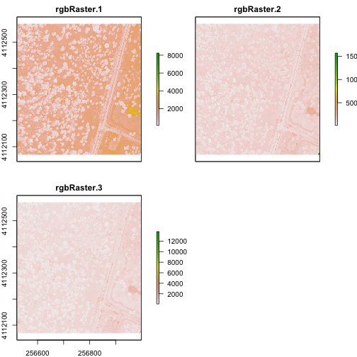
# plot stack
plot(rgbRaster)
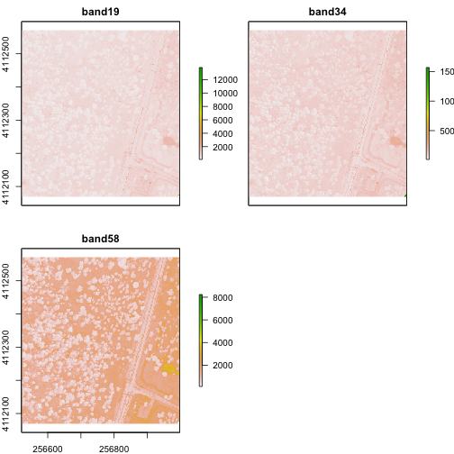
From the attributes we see the CRS, resolution, and extent of all three rasters. The we can see each raster plotted. Notice the different shading between the different bands. This is because the landscape relects in the red, green, and blue spectra differently.
Check out the scale bars. What do they represent?
This reflectance data are radiances corrected for atmospheric effects. The data are typically unitless and ranges from 0-1. NEON Airborne Observation Platform data, where these rasters come from, has a scale factor of 10,000.
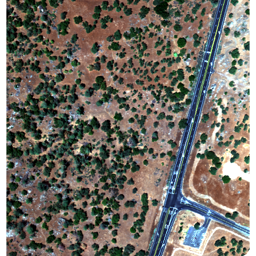
Plot an RGB Image
You can plot a composite RGB image from a raster stack. You need to specify the order of the bands when you do this. In our raster stack, band 19, which is the blue band, is first in the stack, whereas band 58, which is the red band, is last. Thus the order for a RGB image is 3,2,1 to ensure the red band is rendered first as red.
Thinking ahead to next time: If you know you want to create composite RGB images, think about the order of your rasters when you make the stack so the RGB=1,2,3.
We will plot the raster with the rgbRaster() function and the need these
following arguments:
- R object to plot
- which layer of the stack is which color
- stretch: allows for increased contrast. Options are "lin" & "hist".
Let's try it.
# plot an RGB version of the stack
plotRGB(rgbRaster,r=3,g=2,b=1, stretch = "lin")
Note: read the raster package documentation for other arguments that can be
added (like scale) to improve or modify the image.
Explore Raster Values - Histograms
You can also explore the data. Histograms allow us to view the distrubiton of values in the pixels.
# view histogram of reflectance values for all rasters
hist(rgbRaster)

## Warning in .hist1(raster(x, y[i]), maxpixels = maxpixels, main =
## main[y[i]], : 42% of the raster cells were used. 100000 values used.

## Warning in .hist1(raster(x, y[i]), maxpixels = maxpixels, main =
## main[y[i]], : 42% of the raster cells were used. 100000 values used.

## Warning in .hist1(raster(x, y[i]), maxpixels = maxpixels, main =
## main[y[i]], : 42% of the raster cells were used. 100000 values used.
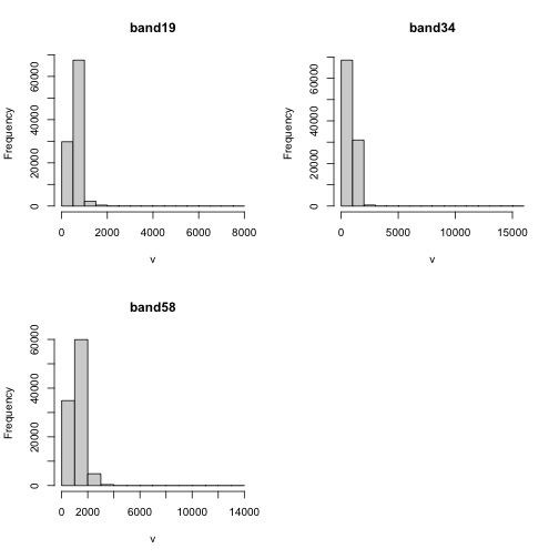
Note about the warning messages: R defaults to only showing the first 100,000 values in the histogram so if you have a large raster you may not be seeing all the values. This saves your from long waits, or crashing R, if you have large datasets.
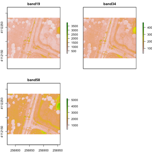
Crop Rasters
You can crop all rasters within a raster stack the same way you'd do it with a single raster.
# determine the desired extent
rgbCrop <- c(256770.7,256959,4112140,4112284)

# crop to desired extent
rgbRaster_crop <- crop(rgbRaster, rgbCrop)

# view cropped stack
plot(rgbRaster_crop)
Raster Bricks in R
In our rgbRaster object we have a list of rasters in a stack. These rasters
are all the same extent, CRS and resolution. By creating a raster brick we
will create one raster object that contains all of the rasters so that we can
use this object to quickly create RGB images. Raster bricks are more efficient
objects to use when processing larger datasets. This is because the computer
doesn't have to spend energy finding the data - it is contained within the object.
# create raster brick
rgbBrick <- brick(rgbRaster)

# check attributes
rgbBrick

## class      : RasterBrick
## dimensions : 502, 477, 239454, 3  (nrow, ncol, ncell, nlayers)
## resolution : 1, 1  (x, y)
## extent     : 256521, 256998, 4112069, 4112571  (xmin, xmax, ymin, ymax)
## crs        : +proj=utm +zone=11 +datum=WGS84 +units=m +no_defs
## source     : memory
## names      : band19, band34, band58
## min values :     84,    116,    123
## max values :  13805,  15677,  14343
While the brick might seem similar to the stack (see attributes above), we can see that it's very different when we look at the size of the object.
- the brick contains all of the data stored in one object
- the stack contains links or references to the files stored on your computer
Use object.size() to see the size of an R object.
# view object size
object.size(rgbBrick)

## 5762000 bytes

object.size(rgbRaster)

## 49984 bytes

# view raster brick
plotRGB(rgbBrick,r=3,g=2,b=1, stretch = "Lin")

Notice the faster plotting? For a smaller raster like this the difference is slight, but for larger raster it can be considerable.
Write to GeoTIFF
We can write out the raster in GeoTIFF format as well. When we do this it will copy the CRS, extent and resolution information so the data will read properly into a GIS program as well. Note that this writes the raster in the order they are in. In our case, the blue (band 19) is first but most programs expect the red band first (RGB).
One way around this is to generate a new raster stack with the rasters in the proper order - red, green and blue format. Or, just always create your stacks R->G->B to start!!!
# Make a new stack in the order we want the data in
orderRGBstack <- stack(rgbRaster$band58,rgbRaster$band34,rgbRaster$band19)

# write the geotiff
# change overwrite=TRUE to FALSE if you want to make sure you don't overwrite your files!
writeRaster(orderRGBstack,paste0(wd,"NEON-DS-Field-Site-Spatial-Data/SJER/RGB/rgbRaster.tif"),"GTiff", overwrite=TRUE)
Import A Multi-Band Image into R
You can import a multi-band image into R too. To do this, you import the file as a stack rather than a raster (which brings in just one band). Let's import the raster than we just created above.
# import multi-band raster as stack
multiRasterS <- stack(paste0(wd,"NEON-DS-Field-Site-Spatial-Data/SJER/RGB/rgbRaster.tif"))

# import multi-band raster direct to brick
multiRasterB <- brick(paste0(wd,"NEON-DS-Field-Site-Spatial-Data/SJER/RGB/rgbRaster.tif"))

# view raster
plot(multiRasterB)
plotRGB(multiRasterB,r=1,g=2,b=3, stretch="lin")

About Hyperspectral Remote Sensing Data
Learning Objectives
After completing this tutorial, you will be able to:
- Define hyperspectral remote sensing.
- Explain the fundamental principles of hyperspectral remote sensing data.
- Describe the key attributes that are required to effectively work with hyperspectral remote sensing data in tools like R, Python, or Google Earth Engine (GEE).
- Describe what a "band" is.
- Define "spectral resolution" and "full width half max (FWHM)".
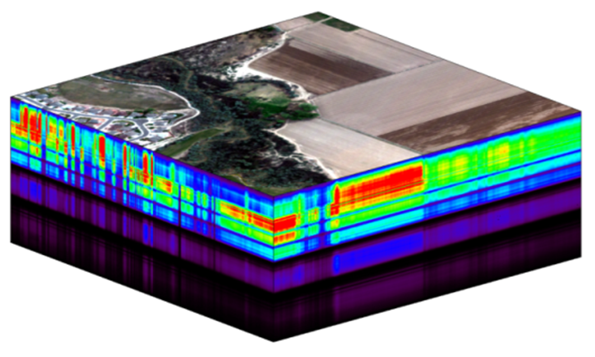
Mapping the Invisible
About Hyperspectral Remote Sensing Data
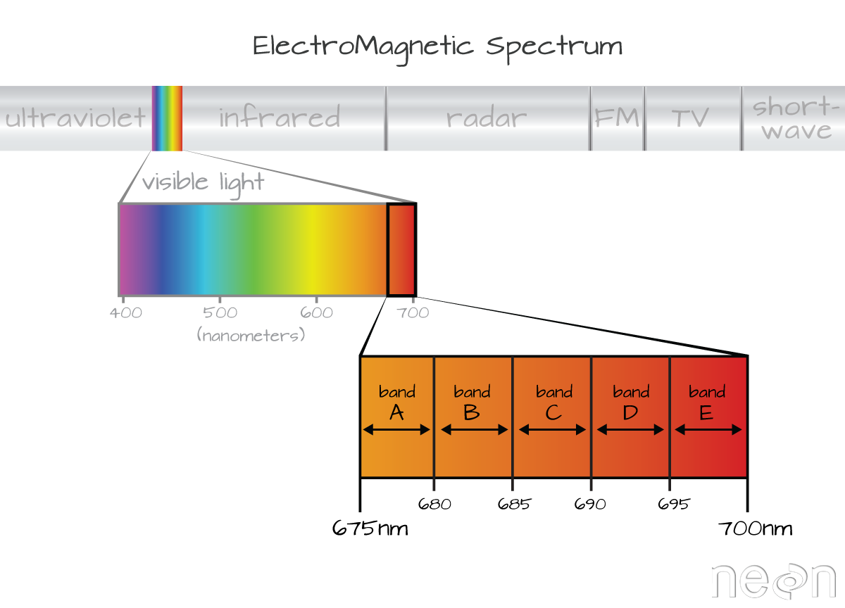
The electromagnetic spectrum is composed of thousands of bands representing different types of light energy. Imaging spectrometers (instruments that collect hyperspectral data) break the electromagnetic spectrum into groups of bands that support classification of objects by their spectral properties on the earth's surface. Hyperspectral data consists of many bands -- up to hundreds of bands -- that cover a portion of the electromagnetic spectrum.
The NEON imaging spectrometer collects data within the 380nm to 2510nm portions of the electromagnetic spectrum within bands that are approximately 5nm in width. This results in a hyperspectral data cube that contains approximately 426 bands - which means big, big data.
Key Metadata for Hyperspectral Data
Bands and Wavelengths
A band represents a group of wavelengths. For example, the wavelength values between 695nm and 700nm might be one band as captured by an imaging spectrometer. The imaging spectrometer collects reflected light energy in a pixel for light in that band. Often when you work with a multi or hyperspectral dataset, the band information is reported as the center wavelength value. This value represents the center point value of the wavelengths represented in that band. Thus in a band spanning 695-700 nm, the center would be 697.5).
Spectral Resolution
The spectral resolution of a dataset that has more than one band, refers to the width of each band in the dataset. In the example above, a band was defined as spanning 695-700nm. The width or spatial resolution of the band is thus 5 nanometers. To see an example of this, check out the band widths for the Landsat sensors.
Full Width Half Max (FWHM)
The full width half max (FWHM) will also often be reported in a multi or hyperspectral dataset. This value represents the spread of the band around that center point.
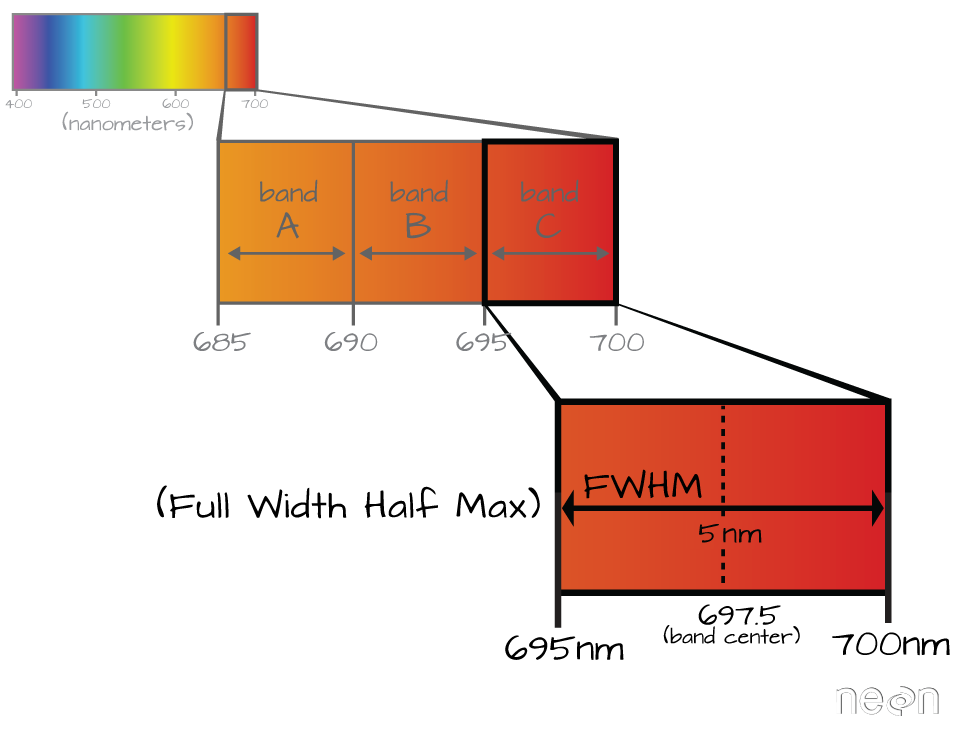
In the illustration above, the band that covers 695-700nm has a FWHM of 5 nm.
While a general spectral resolution of the sensor is often provided, not all sensors create bands of uniform widths. For instance bands 1-9 of Landsat 8 are listed below (Courtesy of USGS)
| Band | Wavelength range (microns) | Spatial Resolution (m) | Spectral Width (microns) |
|---|---|---|---|
| Band 1 - Coastal aerosol | 0.43 - 0.45 | 30 | 0.02 |
| Band 2 - Blue | 0.45 - 0.51 | 30 | 0.06 |
| Band 3 - Green | 0.53 - 0.59 | 30 | 0.06 |
| Band 4 - Red | 0.64 - 0.67 | 30 | 0.03 |
| Band 5 - Near Infrared (NIR) | 0.85 - 0.88 | 30 | 0.03 |
| Band 6 - SWIR 1 | 1.57 - 1.65 | 30 | 0.08 |
| Band 7 - SWIR 2 | 2.11 - 2.29 | 30 | 0.18 |
| Band 8 - Panchromatic | 0.50 - 0.68 | 15 | 0.18 |
| Band 9 - Cirrus | 1.36 - 1.38 | 30 | 0.02 |
Intro to Working with Hyperspectral Remote Sensing Data in HDF5 Format in R
In this tutorial, we will show how to read and extract NEON reflectance data stored within an HDF5 file using R.
Learning Objectives
After completing this tutorial, you will be able to:
- Explain how HDF5 data can be used to store spatial data and the benefits of this format when working with large spatial data cubes.
- Extract metadata from HDF5 files.
- Slice or subset HDF5 data. You will extract one band of pixels.
- Plot a matrix as an image and a raster.
- Export a final GeoTIFF (spatially projected) that can be used both in further analysis and in common GIS tools like QGIS.
Things You’ll Need To Complete This Tutorial
To complete this tutorial you will need the most current version of R and, preferably, RStudio installed on your computer.
As of June 2026, NEON requires an API token for data downloads, to reduce bot scraping and improve user support. Tokens can be generated in NEON data portal user accounts - log in to your account or create one, and go to the API Tokens section. For best practices in storing and using tokens, follow the instructions here.
R Libraries to Install:
-
rhdf5:
install.packages("BiocManager"),BiocManager::install("rhdf5") -
terra:
install.packages("terra") -
neonUtilities:
install.packages("neonUtilities")
More on Packages in R - Adapted from Software Carpentry.
Data to Download
Data will be downloaded in the tutorial using the neonUtilities::byTileAOP() function.
These hyperspectral remote sensing data provide information on the National Ecological Observatory Network's San Joaquin Experimental Range field site in March of 2021. The data were collected over the San Joaquin field site located in California (Domain 17).The entire dataset can be also be downloaded from the NEON Data Portal.
R Script & Challenge Code: NEON data lessons often contain challenges to reinforce skills. If available, the code for challenge solutions is found in the downloadable R script of the entire lesson, available in the footer of each lesson page.
About Hyperspectral Remote Sensing Data
The electromagnetic spectrum is composed of thousands of bands representing different types of light energy. Imaging spectrometers (instruments that collect hyperspectral data) break the electromagnetic spectrum into groups of bands that support classification of objects by their spectral properties on the Earth's surface. Hyperspectral data consists of many bands - up to hundreds of bands - that span a portion of the electromagnetic spectrum, from the visible to the Short Wave Infrared (SWIR) regions.
The NEON imaging spectrometer (NIS) collects data within the 380 nm to 2510 nm portions of the electromagnetic spectrum within bands that are approximately 5 nm in width. This results in a hyperspectral data cube that contains approximately 426 bands - which means BIG DATA.
The HDF5 data model natively compresses data stored within it (makes it smaller) and supports data slicing (extracting only the portions of the data that you need to work with rather than reading the entire dataset into memory). These features make it ideal for working with large data cubes such as those generated by imaging spectrometers, in addition to supporting spatial data and associated metadata.
In this tutorial we will demonstrate how to read and extract spatial raster data stored within an HDF5 file using R.
Read HDF5 data into R
We will use the terra and rhdf5 packages to read in the HDF5 file that contains hyperspectral data for the NEON San Joaquin (SJER) field site.
Let's start by calling the needed packages and reading in our NEON HDF5 file.
Please be sure that you have at least version 2.10 of rhdf5 installed. Use:
packageVersion("rhdf5") to check the package version.
Data Tip: To update all packages installed in R, use update.packages().
# Load `terra` and `rhdf5` packages to read NIS data into R

library(terra)

library(rhdf5)

library(neonUtilities)

# Read in NEON_TOKEN (see "Things You'll Need to Complete This Tutorial" section to set this up)

token <- Sys.getenv("NEON_TOKEN")
Set the working directory to ensure R can find the file we are importing, and we know where the file is being saved. You can move the file that is downloaded afterward, but be sure to re-set the path to the file.
data_dir <- "~/data/" #This will depend on your local environment
We can use the neonUtilities function byTileAOP to download a single reflectance tile. You can run help(byTileAOP) to see more details on what the various inputs are. For this exercise, we'll specify the UTM Easting and Northing to be (257500, 4112500), which will download the tile with the lower left corner (257000,4112000). By default, the function will check the size total size of the download and ask you whether you wish to proceed (y/n). This file is ~672.7 MB, so make sure you have enough space on your local drive. You can set check.size=FALSE if you want to download without a prompt.
byTileAOP(dpID='DP3.30006.001',

          site='SJER',

          year='2021',

          easting=257500,

          northing=4112500,

          check.size=TRUE, # set to FALSE if you don't want to enter y/n

          savepath = data_dir,

          token=token)
This file will be downloaded into a nested subdirectory under the ~/data folder, inside a folder named DP3.30006.001 (the Data Product ID). The file should show up in this location: ~/data/DP3.30006.001/neon-aop-products/2021/FullSite/D17/2021_SJER_5/L3/Spectrometer/Reflectance/NEON_D17_SJER_DP3_257000_4112000_reflectance.h5.
Data Tip: To make sure you are pointing to the correct path, look in the ~/data folder and navigate to where the .h5 file is saved, or use the R command list.files(path=data_dir,pattern="\\.h5$",recursive=TRUE,full.names=TRUE) to display the full path of the .h5 file. Note, if you have any other .h5 files downloaded in this folder, it will display all of the hdf5 files.
# Define the h5 file name to be opened

h5_file <- paste0(data_dir,"DP3.30006.001/neon-aop-products/2021/FullSite/D17/2021_SJER_5/L3/Spectrometer/Reflectance/NEON_D17_SJER_DP3_257000_4112000_reflectance.h5")
You can use h5ls and/or View(h5ls(...)) to look at the contents of the hdf5 file, as follows:
# look at the HDF5 file structure

View(h5ls(h5_file,all=T))
When you look at the structure of the data, take note of the "map info" dataset, the Coordinate_System group, and the wavelength and Reflectance datasets. The Coordinate_System folder contains the spatial attributes of the data including its EPSG Code, which is easily converted to a Coordinate Reference System (CRS). The CRS documents how the data are physically located on the Earth. The wavelength dataset contains the wavelength values for each band in the data. The Reflectance dataset contains the image data that we will use for both data processing and visualization.
More Information on raster metadata:
-
Raster Data in R - The Basics - this tutorial explains more about how rasters work in R and their associated metadata.
-
About Hyperspectral Remote Sensing Data -this tutorial explains more about metadata and important concepts associated with multi-band (multi and hyperspectral) rasters.
Data Tip - HDF5 Structure: Note that the structure of individual HDF5 files may vary depending on who produced the data. In this case, the Wavelength and reflectance data within the file are both h5 datasets. However, the spatial information is contained within a group. Data downloaded from another organization (like NASA) may look different. This is why it's important to explore the data as a first step!
We can use the h5readAttributes() function to read and extract metadata from the HDF5 file. Let's start by learning about the wavelengths described within this file.
# get information about the wavelengths of this dataset

wavelengthInfo <- h5readAttributes(h5_file,"/SJER/Reflectance/Metadata/Spectral_Data/Wavelength")

wavelengthInfo

## $Description
## [1] "Central wavelength of the reflectance bands."
##
## $Units
## [1] "nanometers"
Next, we can use the h5read function to read the data contained within the HDF5 file. Let's read in the wavelengths of the band centers:
# read in the wavelength information from the HDF5 file

wavelengths <- h5read(h5_file,"/SJER/Reflectance/Metadata/Spectral_Data/Wavelength")

head(wavelengths)

## [1] 381.6035 386.6132 391.6229 396.6327 401.6424 406.6522

tail(wavelengths)

## [1] 2485.693 2490.703 2495.713 2500.722 2505.732 2510.742
Which wavelength is band 21 associated with?
(Hint: look at the wavelengths vector that we just imported and check out the data located at index 21 - wavelengths[21]).
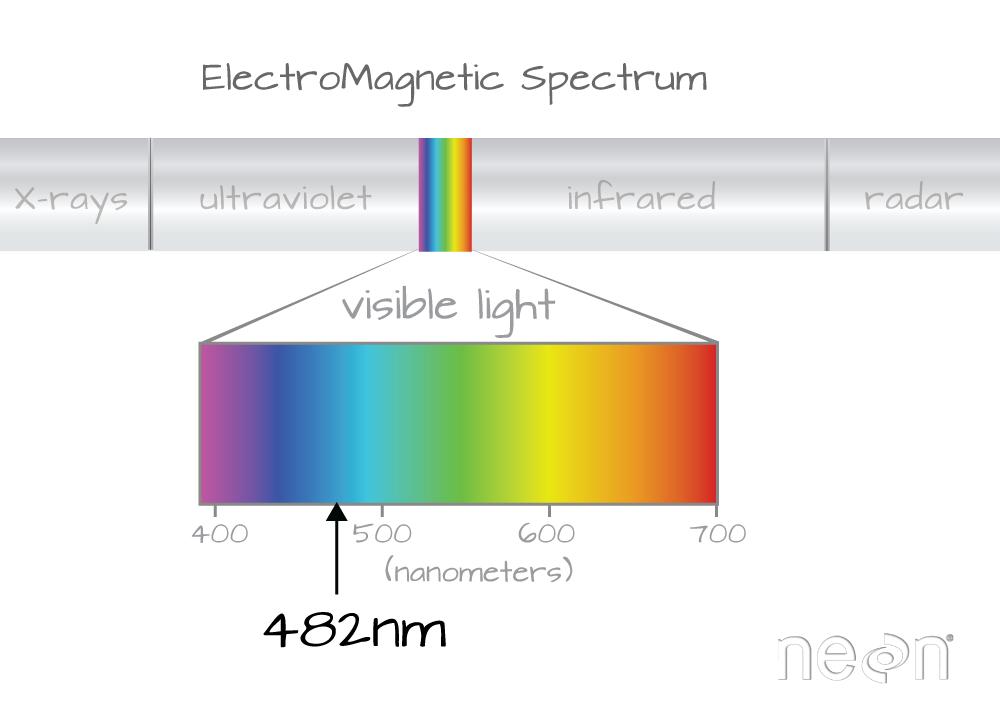
Band 21 has a associated wavelength center of 481.7982 nanometers (nm) which is in the blue portion (~380-500 nm) of the visible electromagnetic spectrum (~380-700 nm).
Bands and Wavelengths
A band represents a group of wavelengths. For example, the wavelength values between 695 nm and 700 nm might be one band captured by an imaging spectrometer. The imaging spectrometer collects reflected light energy in a pixel for light in that band. Often when you work with a multi- or hyperspectral dataset, the band information is reported as the center wavelength value. This value represents the mean value of the wavelengths represented in that band. Thus in a band spanning 695-700 nm, the center would be 697.5 nm). The full width half max (FWHM) will also be reported. This value can be thought of as the spread of the band around that center point. So, a band that covers 800-805 nm might have a FWHM of 5 nm and a wavelength value of 802.5 nm.

The HDF5 dataset that we are working with in this activity may contain more information than we need to work with. For example, we don't necessarily need to process all 426 bands available in a full NEON hyperspectral reflectance file - if we are interested in creating a product like NDVI which only uses bands in the Near InfraRed (NIR) and Red portions of the spectrum. Or we might only be interested in a spatial subset of the data - perhaps an area where we have collected corresponding ground data in the field.
The HDF5 format allows us to slice (or subset) the data - quickly extracting the subset that we need to process. Let's extract one of the green bands - band 34.
By the way - what is the center wavelength value associated with band 34?
Hint: wavelengths[34].
How do we know this band is a green band in the visible portion of the spectrum?
In order to effectively subset our data, let's first read the reflectance metadata stored as attributes in the "Reflectance_Data" dataset.
# First, we need to extract the reflectance metadata:

reflInfo <- h5readAttributes(h5_file, "/SJER/Reflectance/Reflectance_Data")

reflInfo

## $Cloud_conditions
## [1] "For cloud conditions information see Weather Quality Index dataset."
##
## $Cloud_type
## [1] "Cloud type may have been selected from multiple flight trajectories."
##
## $Data_Ignore_Value
## [1] -9999
##
## $Description
## [1] "Atmospherically corrected reflectance."
##
## $Dimension_Labels
## [1] "Line, Sample, Wavelength"
##
## $Dimensions
## [1] 1000 1000  426
##
## $Interleave
## [1] "BSQ"
##
## $Scale_Factor
## [1] 10000
##
## $Spatial_Extent_meters
## [1]  257000  258000 4112000 4113000
##
## $Spatial_Resolution_X_Y
## [1] 1 1
##
## $Units
## [1] "Unitless."
##
## $Units_Valid_range
## [1]     0 10000

# Next, we read the different dimensions


nRows <- reflInfo$Dimensions[1]

nCols <- reflInfo$Dimensions[2]

nBands <- reflInfo$Dimensions[3]


nRows

## [1] 1000

nCols

## [1] 1000

nBands

## [1] 426
The HDF5 read function reads data in the order: Bands, Cols, Rows. This is different from how R reads data. We'll adjust for this later.
# Extract or "slice" data for band 34 from the HDF5 file

b34 <- h5read(h5_file,"/SJER/Reflectance/Reflectance_Data",index=list(34,1:nCols,1:nRows))


# what type of object is b34?

class(b34)

## [1] "array"
A Note About Data Slicing in HDF5
Data slicing allows us to extract and work with subsets of the data rather than reading in the entire dataset into memory. In this example, we will extract and plot the green band without reading in all 426 bands. The ability to slice large datasets makes HDF5 ideal for working with big data.
Next, let's convert our data from an array (more than 2 dimensions) to a matrix (just 2 dimensions). We need to have our data in a matrix format to plot it.
# convert from array to matrix by selecting only the first band

b34 <- b34[1,,]


# display the class of this re-defined variable

class(b34)

## [1] "matrix" "array"
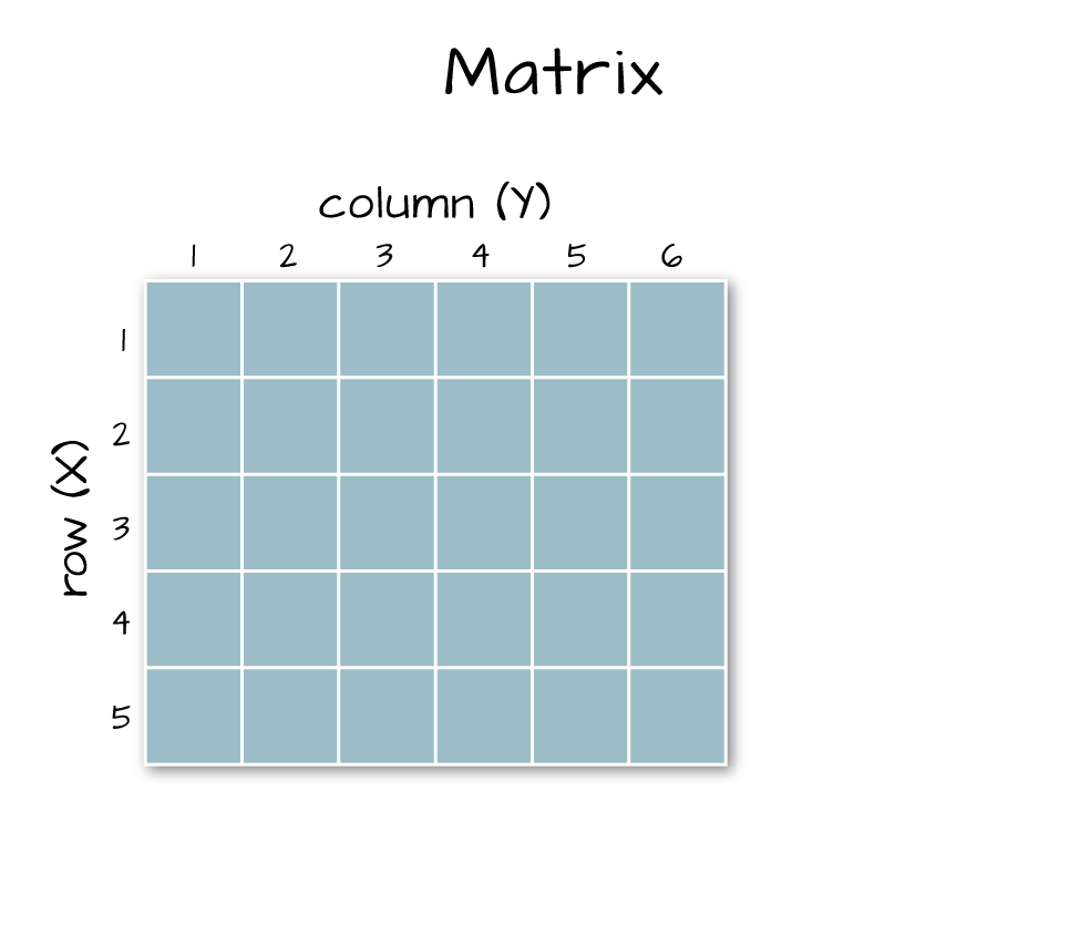
Arrays vs. Matrices
Arrays are matrices with more than 2 dimensions. When we say dimension, we are talking about the "z" associated with the data (imagine a series of tabs in a spreadsheet). Put the other way: matrices are arrays with only 2 dimensions. Arrays can have any number of dimensions one, two, ten or more.
Here is a matrix that is 4 x 3 in size (4 rows and 3 columns):
| Metric | species 1 | species 2 |
|---|---|---|
| total number | 23 | 45 |
| average weight | 14 | 5 |
| average length | 2.4 | 3.5 |
| average height | 32 | 12 |
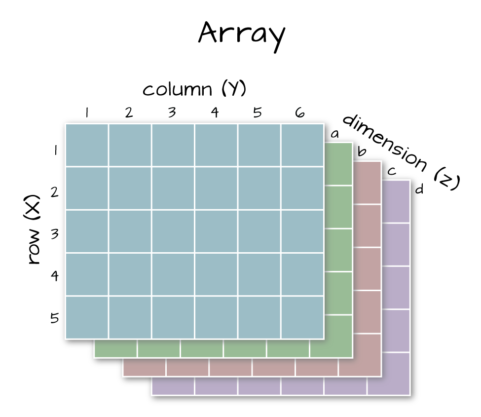
Dimensions in Arrays
An array contains 1 or more dimensions in the "z" direction. For example, let's say that we collected the same set of species data for every day in a 30 day month. We might then have a matrix like the one above for each day for a total of 30 days making a 4 x 3 x 30 array (this dataset has more than 2 dimensions). More on R object types here (links to external site, DataCamp).
Next, let's look at the metadata for the reflectance data. When we do this, take note of 1) the scale factor and 2) the data ignore value. Then we can plot the band 34 data. Plotting spatial data as a visual "data check" is a good idea to make sure processing is being performed correctly and all is well with the image.
# look at the metadata for the reflectance dataset

h5readAttributes(h5_file,"/SJER/Reflectance/Reflectance_Data")

## $Cloud_conditions
## [1] "For cloud conditions information see Weather Quality Index dataset."
##
## $Cloud_type
## [1] "Cloud type may have been selected from multiple flight trajectories."
##
## $Data_Ignore_Value
## [1] -9999
##
## $Description
## [1] "Atmospherically corrected reflectance."
##
## $Dimension_Labels
## [1] "Line, Sample, Wavelength"
##
## $Dimensions
## [1] 1000 1000  426
##
## $Interleave
## [1] "BSQ"
##
## $Scale_Factor
## [1] 10000
##
## $Spatial_Extent_meters
## [1]  257000  258000 4112000 4113000
##
## $Spatial_Resolution_X_Y
## [1] 1 1
##
## $Units
## [1] "Unitless."
##
## $Units_Valid_range
## [1]     0 10000

# plot the image

image(b34)
What do you notice about the first image? It's washed out and lacking any detail. What could be causing this? It got better when plotting the log of the values, but still not great.
# this is a little hard to visually interpret - what happens if we plot a log of the data?

image(log(b34))
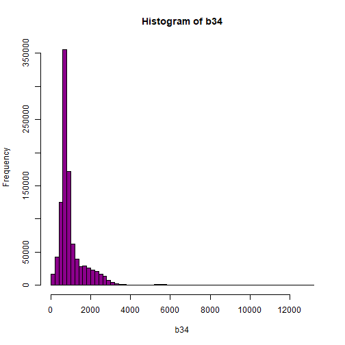
Let's look at the distribution of reflectance values in our data to figure out what is going on.
# Plot range of reflectance values as a histogram to view range

# and distribution of values.

hist(b34,breaks=50,col="darkmagenta")
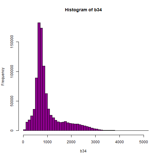
# View values between 0 and 5000

hist(b34,breaks=100,col="darkmagenta",xlim = c(0, 5000))
# View higher values

hist(b34, breaks=100,col="darkmagenta",xlim = c(5000, 15000),ylim = c(0, 750))
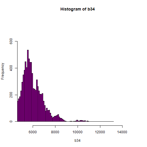
As you're examining the histograms above, keep in mind that reflectance values range between 0-1. The data scale factor in the metadata tells us to divide all reflectance values by 10,000. Thus, a value of 5,000 equates to a reflectance value of 0.50. Storing data as integers (without decimal places) compared to floating points (with decimal places) creates a smaller file. This type of scaling is commin in remote sensing datasets.
Notice in the data that there are some larger reflectance values (>5,000) that represent a smaller number of pixels. These pixels are skewing how the image renders.
Data Ignore Value
Image data in raster format will often contain a data ignore value and a scale factor. The data ignore value represents pixels where there are no data. Among other causes, no data values may be attributed to the sensor not collecting data in that area of the image or to processing results which yield null values.
Remember that the metadata for the Reflectance dataset designated -9999 as data ignore value. Thus, let's set all pixels with a value == -9999 to NA (no value). If we do this, R won't render these pixels.
# there is a no data value in our raster - let's define it

noDataValue <- as.numeric(reflInfo$Data_Ignore_Value)

noDataValue

## [1] -9999

# set all values equal to the no data value (-9999) to NA

b34[b34 == noDataValue] <- NA


# plot the image now

image(b34)

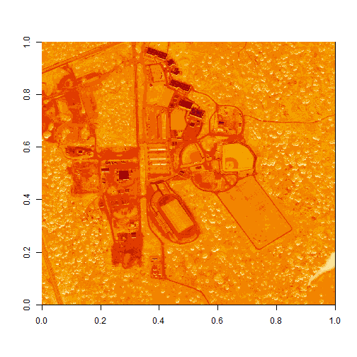
Reflectance Values and Image Stretch
Our image still looks dark because R is trying to render all reflectance values between 0 and 14999 as if they were distributed equally in the histogram. However we know they are not distributed equally. There are many more values between 0-5000 than there are values >5000.
Images contain a distribution of reflectance values. A typical image viewing program will render the values by distributing the entire range of reflectance values across a range of "shades" that the monitor can render - between 0 and 255. However, often the distribution of reflectance values is not linear. For example, in the case of our data, most of the reflectance values fall between 0 and 0.5. Yet there are a few values >0.8 that are heavily impacting the way the image is drawn on our monitor. Imaging processing programs like ENVI, QGIS and ArcGIS (and even Adobe Photoshop) allow you to adjust the stretch of the image. This is similar to adjusting the contrast and brightness in Photoshop.
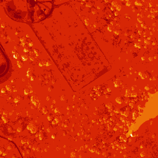
The proper way to adjust our data would be to apply what's called an image stretch. We will learn how to stretch our image data later. For now, let's plot the values as the log function on the pixel reflectance values to factor out those larger values.
image(log(b34))

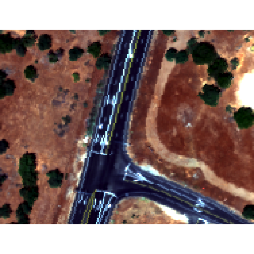
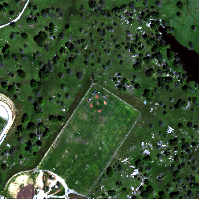
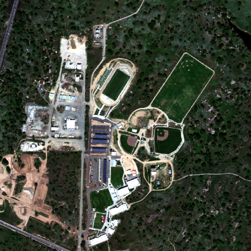
The log applied to our image increases the contrast making it look more like an image. However, look at the images below. The top one is an RGB image as the image should look. The bottom one is our log-adjusted image. Notice a difference?
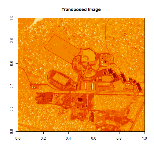
Transpose Image
Notice that there are three data dimensions for this file: Bands x Rows x Columns. However, when R reads in the dataset, it reads them as: Columns x Bands x Rows. The data are flipped. We can quickly transpose the data to correct for this using the t or transpose command in R.
The orientation is rotated in our log adjusted image. This is because R reads in matrices starting from the upper left hand corner. While most rasters read pixels starting from the lower left hand corner. In the next section, we will deal with this issue by creating a proper georeferenced (spatially located) raster in R. The raster format will read in pixels following the same methods as other GIS and imaging processing software like QGIS and ENVI do.
# We need to transpose x and y values in order for our

# final image to plot properly

b34 <- t(b34)

image(log(b34), main="Transposed Image")
Create a Georeferenced Raster
Next, we will create a proper raster using the b34 matrix. The raster format will allow us to define and manage:
- Image stretch
- Coordinate reference system & spatial reference
- Resolution
- and other raster attributes...
It will also account for the orientation issue discussed above.
To create a raster in R, we need a few pieces of information, including:
- The coordinate reference system (CRS)
- The spatial extent of the image
Define Raster CRS
First, we need to define the Coordinate reference system (CRS) of the raster. To do that, we can first grab the EPSG code from the HDF5 attributes, and covert the EPSG to a CRS string. Then we can assign that CRS to the raster object.
# Extract the EPSG from the h5 dataset
h5EPSG <- h5read(h5_file, "/SJER/Reflectance/Metadata/Coordinate_System/EPSG Code")
# convert the EPSG code to a CRS string
h5CRS <- crs(paste0("+init=epsg:",h5EPSG))
# define final raster with projection info
# note that capitalization will throw errors on a MAC.
# if UTM is all caps it might cause an error!
b34r <- rast(b34,
crs=h5CRS)
# view the raster attributes
b34r
## class : SpatRaster
## size : 1000, 1000, 1 (nrow, ncol, nlyr)
## resolution : 1, 1 (x, y)
## extent : 0, 1000, 0, 1000 (xmin, xmax, ymin, ymax)
## coord. ref. : WGS 84 / UTM zone 11N
## source(s) : memory
## name : lyr.1
## min value : 32
## max value : 13129
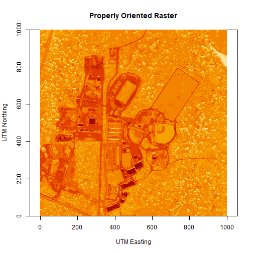
# let's have a look at our properly oriented raster. Take note of the
# coordinates on the x and y axis.
image(log(b34r),
xlab = "UTM Easting",
ylab = "UTM Northing",
main = "Properly Oriented Raster")
Next we define the extents of our raster. The extents will be used to calculate the raster's resolution. Fortunately, the spatial extent is provided in the HDF5 file "Reflectance_Data" group attributes that we saved before as reflInfo.
# Grab the UTM coordinates of the spatial extent

xMin <- reflInfo$Spatial_Extent_meters[1]

xMax <- reflInfo$Spatial_Extent_meters[2]

yMin <- reflInfo$Spatial_Extent_meters[3]

yMax <- reflInfo$Spatial_Extent_meters[4]


# define the extent (left, right, top, bottom)

rasExt <- ext(xMin,xMax,yMin,yMax)

rasExt

## SpatExtent : 257000, 258000, 4112000, 4113000 (xmin, xmax, ymin, ymax)

# assign the spatial extent to the raster

ext(b34r) <- rasExt


# look at raster attributes

b34r

## class       : SpatRaster
## size        : 1000, 1000, 1  (nrow, ncol, nlyr)
## resolution  : 1, 1  (x, y)
## extent      : 257000, 258000, 4112000, 4113000  (xmin, xmax, ymin, ymax)
## coord. ref. : WGS 84 / UTM zone 11N
## source(s)   : memory
## name        : lyr.1
## min value   :    32
## max value   : 13129
Learn more about working with Raster data in R in the Data Carpentry workshop: Introduction to Geospatial Raster and Vector Data with R.
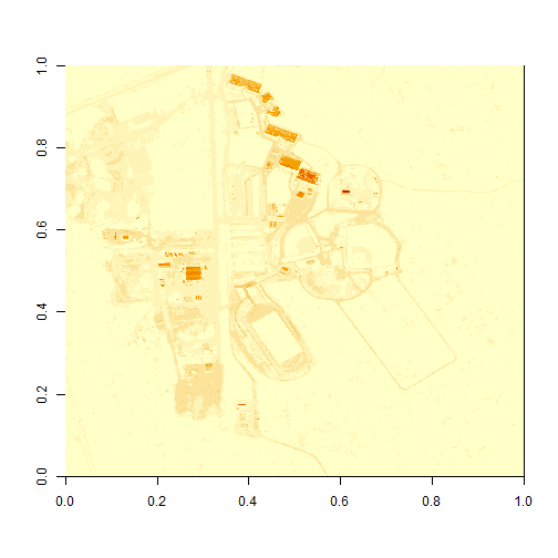
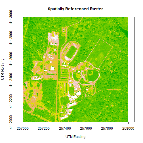
We can adjust the colors of our raster as well, if desired.
# let's change the colors of our raster and adjust the zlim

col <- terrain.colors(25)


image(b34r,
      xlab = "UTM Easting",
      ylab = "UTM Northing",
      main= "Spatially Referenced Raster",
      col=col,
      zlim=c(0,3000))
We've now created a raster from band 34 reflectance data. We can export the data as a raster, using the writeRaster command. Note that it's good practice to close the H5 connection before moving on!
# write out the raster as a geotiff

writeRaster(b34r,

            file=paste0(data_dir,"band34.tif"),

            overwrite=TRUE)


# close the H5 file

H5close()
Challenge: Work with Rasters
Try these three extensions on your own:
-
Create rasters using other bands in the dataset.
-
Vary the distribution of values in the image to mimic an image stretch. e.g.
b34[b34 > 6000 ] <- 6000 -
Use what you know to extract ALL of the reflectance values for ONE pixel rather than for an entire band. HINT: this will require you to pick an x and y value and then all values in the z dimension:
aPixel<- h5read(h5_file,"Reflectance",index=list(NULL,100,35)). Plot the spectra output.
Creating a Raster Stack from Hyperspectral Imagery in HDF5 Format in R
In this tutorial, we will learn how to create multi (3) band images from hyperspectral data. We will also learn how to perform some basic raster calculations (known as raster math in the GIS world).
Learning Objectives
After completing this activity, you will be able to:
- Extract a "slice" of data from a hyperspectral data cube.
- Create a raster "stack" in R which can be used to create RGB images from band combinations in a hyperspectral data cube.
- Plot data spatially on a map.
- Create basic vegetation indices like NDVI using raster-based calculations in R.
Things You’ll Need To Complete This Tutorial
To complete this tutorial you will need the most current version of R and, preferably, RStudio loaded on your computer. You will also need to create a NEON API token.
R Libraries to Install:
-
rhdf5:
install.packages("BiocManager"),BiocManager::install("rhdf5") -
terra:
install.packages("terra") -
neonUtilities:
install.packages("neonUtilities")
More on Packages in R - Adapted from Software Carpentry.
Data
These hyperspectral remote sensing data provide information on the National Ecological Observatory Network's San Joaquin Experimental Range (SJER) field site in March of 2021. The data used in this lesson is the 1km by 1km mosaic tile named NEON_D17_SJER_DP3_257000_4112000_reflectance.h5. If you already completed the previous lesson in this tutorial series, you do not need to download this data again. The entire SJER reflectance dataset can be accessed from the NEON Data Portal.
R Script & Challenge Code: NEON data lessons often contain challenges to reinforce skills. If available, the code for challenge solutions is found in the downloadable R script of the entire lesson, available in the footer of each lesson page.
Recommended Skills
For this tutorial you should be comfortable working with HDF5 files that contain hyperspectral data, including reading in reflectance values and associated metadata and attributes.
If you aren't familiar with these steps already, we highly recommend you work through the Introduction to Working with Hyperspectral Data in HDF5 Format in R tutorial before moving on to this tutorial.
About Hyperspectral Data
We often want to generate a 3 band image from multi or hyperspectral data. The most commonly recognized band combination is RGB which stands for Red, Green and Blue. RGB images are just like an image that your camera takes. But other band combinations can be useful too. For example, near infrared images highlight healthy vegetation, which makes it easy to classify or identify where vegetation is located on the ground.
Data Tip - Band Combinations: The Biodiversity Informatics group created a great interactive tool that lets you explore band combinations. Check it out. Learn more about band combinations using a great online tool from the American Museum of Natural History! (The tool requires Flash player.)
Create a Raster Stack in R
In the previous lesson, we exported a single band of the NEON Reflectance data from a HDF5 file. In this activity, we will create a full color image using 3 (red, green and blue - RGB) bands. We will follow many of the steps we followed in the Intro to Working with Hyperspectral Remote Sensing Data in HDF5 Format in R tutorial. These steps included loading required packages, downloading the data (optionally, you don't need to do this if you downloaded the data from the previous lesson), and reading in our file and viewing the hdf5 file structure.
First, let's load the required R packages, terra and rhdf5, and read in our token.
As of June 2026, NEON requires an API token for data downloads, to reduce bot scraping and improve user support. Tokens can be generated in NEON data portal user accounts - log in to your account or create one, and go to the API Tokens section. For best practices in storing and using tokens, follow the instructions here.
library(terra)
library(rhdf5)
library(neonUtilities)

token <- Sys.getenv("NEON_TOKEN")
Next set the working directory to ensure R can find the file we wish to import. Be sure to move the download into your working directory!
# set data directory (this will depend on your local environment)
data_dir <- "~/data/"
We can use the neonUtilities function byTileAOP to download a single reflectance tile. You can run help(byTileAOP) to see more details on what the various inputs are. For this exercise, we'll specify the UTM Easting and Northing to be (257500, 4112500), which will download the tile with the lower left corner (257000, 4112000).
byTileAOP(dpID = 'DP3.30006.001',
          site = 'SJER',
          year = '2021',
          easting = 257500,
          northing = 4112500,
          savepath = data_dir,
          token=token)

## Downloading 1 files

##
|
| | 0%
|
|======================================================================================| 100%
## Successfully downloaded 1 files to ~/data//DP3.30006.001
This file will be downloaded into a nested subdirectory under the ~/data folder, inside a folder named DP3.30006.001 (the Data Product ID). The file should show up in this location: ~/data/DP3.30006.001/neon-aop-products/2021/FullSite/D17/2021_SJER_5/L3/Spectrometer/Reflectance/NEON_D17_SJER_DP3_257000_4112000_reflectance.h5.
Now we can read in the file. You can move this file to a different location, but make sure to change the path accordingly.
# Define the h5 file name to be opened

h5_file <- paste0(data_dir,"DP3.30006.001/neon-aop-products/2021/FullSite/D17/2021_SJER_5/L3/Spectrometer/Reflectance/NEON_D17_SJER_DP3_257000_4112000_reflectance.h5")
As in the last lesson, let's use View(h5ls) to take a look inside this hdf5 dataset:
View(h5ls(h5_file,all=T))
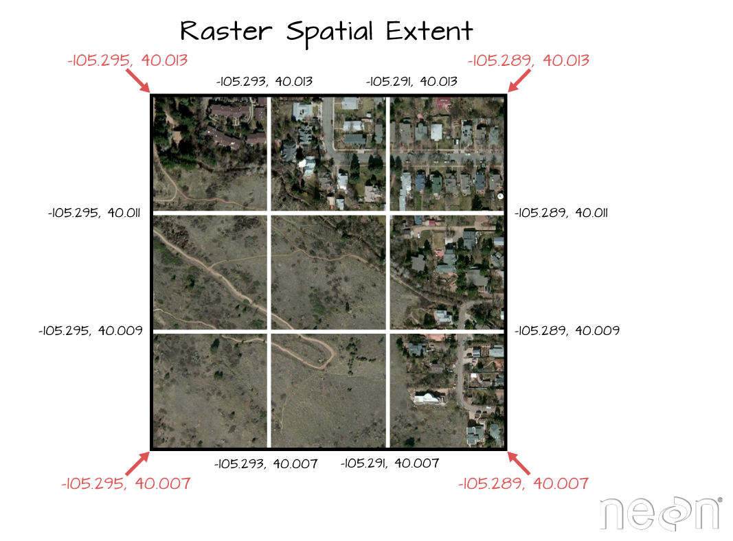
To spatially locate our raster data, we need a few key attributes:
- The coordinate reference system
- The spatial extent of the raster
We'll begin by grabbing these key attributes from the H5 file.
# define coordinate reference system from the EPSG code provided in the HDF5 file
h5EPSG <- h5read(h5_file,"/SJER/Reflectance/Metadata/Coordinate_System/EPSG Code" )
h5CRS <- crs(paste0("+init=epsg:",h5EPSG))

# get the Reflectance_Data attributes
reflInfo <- h5readAttributes(h5_file,"/SJER/Reflectance/Reflectance_Data" )

# Grab the UTM coordinates of the spatial extent
xMin <- reflInfo$Spatial_Extent_meters[1]
xMax <- reflInfo$Spatial_Extent_meters[2]
yMin <- reflInfo$Spatial_Extent_meters[3]
yMax <- reflInfo$Spatial_Extent_meters[4]

# define the extent (left, right, top, bottom)
rastExt <- ext(xMin,xMax,yMin,yMax)

# view the extent to make sure that it looks right
rastExt

## SpatExtent : 257000, 258000, 4112000, 4113000 (xmin, xmax, ymin, ymax)

# Finally, define the no data value for later
h5NoDataValue <- as.integer(reflInfo$Data_Ignore_Value)
cat('No Data Value:',h5NoDataValue)

## No Data Value: -9999
Next, we'll write a function that will perform the processing that we did step by step in the Intro to Working with Hyperspectral Remote Sensing Data in HDF5 Format in R. This will allow us to process multiple bands in bulk.
The function band2Rast slices a band of data from the HDF5 file, and extracts the reflectance array for that band. It then converts the data into a matrix, converts it to a raster, and finally returns a spatially corrected raster for the specified band.
The function requires the following variables:
- file: the hdf5 reflectance file
- band: the band number we wish to extract
- noDataValue: the noDataValue for the raster
-
extent: a terra spatial extent (
SpatExtent) object . - crs: the Coordinate Reference System for the raster
The function output is a spatially referenced, R terra object.
# file: the hdf5 file
# band: the band you want to process
# returns: a matrix containing the reflectance data for the specific band

band2Raster <- function(file, band, noDataValue, extent, CRS){
    # first, read in the raster
    out <- h5read(file,"/SJER/Reflectance/Reflectance_Data",index=list(band,NULL,NULL))
	  # Convert from array to matrix
	  out <- (out[1,,])
	  # transpose data to fix flipped row and column order
    # depending upon how your data are formatted you might not have to perform this
    # step.
	  out <- t(out)
    # assign data ignore values to NA
    # note, you might chose to assign values of 15000 to NA
    out[out == noDataValue] <- NA

    # turn the out object into a raster
    outr <- rast(out,crs=CRS)

    # assign the extents to the raster
    ext(outr) <- extent

    # return the terra raster object
    return(outr)
}
Now that the function is created, we can create our list of rasters. The list specifies which bands (or dimensions in our hyperspectral dataset) we want to include in our raster stack. Let's start with a typical RGB (red, green, blue) combination. We will use bands 14, 9, and 4 (bands 58, 34, and 19 in a full NEON hyperspectral dataset).
Data Tip - wavelengths and bands: Remember that you can look at the wavelengths dataset in the HDF5 file to determine the center wavelength value for each band. Keep in mind that this data subset only includes every fourth band that is available in a full NEON hyperspectral dataset!
# create a list of the bands (R,G,B) we want to include in our stack
rgb <- list(58,34,19)

# lapply tells R to apply the function to each element in the list

rgb_rast <- lapply(rgb,FUN=band2Raster, file = h5_file,
                   noDataValue=h5NoDataValue,
                   ext=rastExt,
                   CRS=h5CRS)
Check out the properties or rgb_rast:
rgb_rast

## [[1]]
## class       : SpatRaster
## size        : 1000, 1000, 1  (nrow, ncol, nlyr)
## resolution  : 1, 1  (x, y)
## extent      : 257000, 258000, 4112000, 4113000  (xmin, xmax, ymin, ymax)
## coord. ref. : WGS 84 / UTM zone 11N
## source(s)   : memory
## name        : lyr.1
## min value   :     0
## max value   : 14950
##
## [[2]]
## class       : SpatRaster
## size        : 1000, 1000, 1  (nrow, ncol, nlyr)
## resolution  : 1, 1  (x, y)
## extent      : 257000, 258000, 4112000, 4113000  (xmin, xmax, ymin, ymax)
## coord. ref. : WGS 84 / UTM zone 11N
## source(s)   : memory
## name        : lyr.1
## min value   :    32
## max value   : 13129
##
## [[3]]
## class       : SpatRaster
## size        : 1000, 1000, 1  (nrow, ncol, nlyr)
## resolution  : 1, 1  (x, y)
## extent      : 257000, 258000, 4112000, 4113000  (xmin, xmax, ymin, ymax)
## coord. ref. : WGS 84 / UTM zone 11N
## source(s)   : memory
## name        : lyr.1
## min value   :     9
## max value   : 11802
Note that it displays properties of 3 rasters. Finally, we can create a raster stack from our list of rasters as follows:
rgbStack <- rast(rgb_rast)
In the code chunk above, we used the lapply() function, which is a powerful, flexible way to apply a function (in this case, our band2Raster() function) multiple times. You can learn more about lapply() here.
NOTE: We are using the raster stack object in R to store several rasters that are of the same CRS and extent. This is a popular and convenient way to organize co-incident rasters.
Next, add the names of the bands to the raster so we can easily keep track of the bands in the list.
# Create a list of band names
bandNames <- paste("Band_",unlist(rgb),sep="")

# set the rasterStack's names equal to the list of bandNames created above
names(rgbStack) <- bandNames

# check properties of the raster list - note the band names
rgbStack

## class       : SpatRaster
## size        : 1000, 1000, 3  (nrow, ncol, nlyr)
## resolution  : 1, 1  (x, y)
## extent      : 257000, 258000, 4112000, 4113000  (xmin, xmax, ymin, ymax)
## coord. ref. : WGS 84 / UTM zone 11N
## source(s)   : memory
## names       : Band_58, Band_34, Band_19
## min values  :       0,      32,       9
## max values  :   14950,   13129,   11802


# scale the data as specified in the reflInfo$Scale Factor
rgbStack <- rgbStack/as.integer(reflInfo$Scale_Factor)

# plot one raster in the stack to make sure things look OK.
plot(rgbStack$Band_58, main="Band 58")
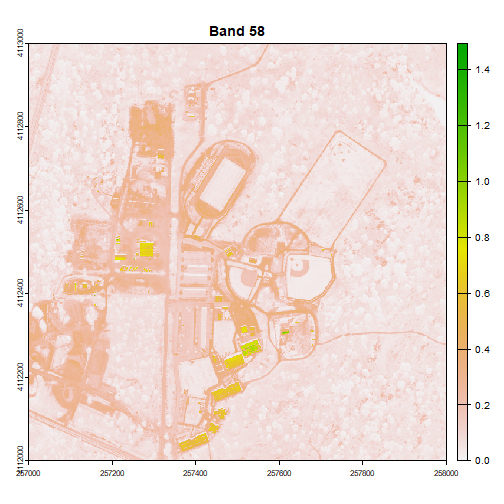
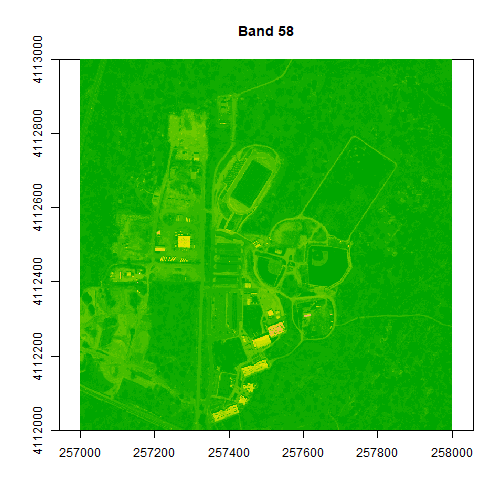
We can play with the color ramps too if we want:
# change the colors of our raster
colors1 <- terrain.colors(25)
image(rgbStack$Band_58, main="Band 58", col=colors1)
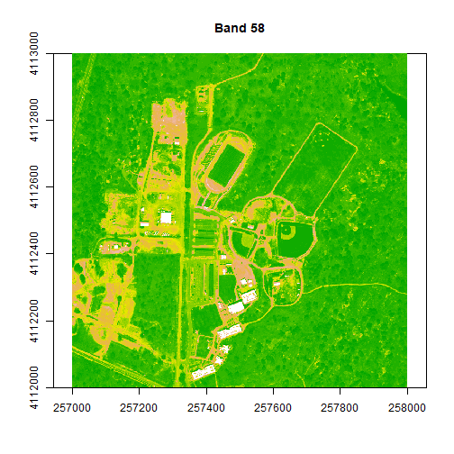
# adjust the zlims or the stretch of the image
image(rgbStack$Band_58, main="Band 58", col=colors1, zlim = c(0,.5))
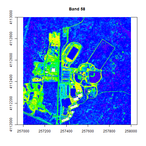
# try a different color palette
colors2 <- topo.colors(15, alpha = 1)
image(rgbStack$Band_58, main="Band 58", col=colors2, zlim=c(0,.5))
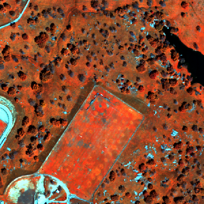
The plotRGB function allows you to combine three bands to create an true-color image.
# create a 3 band RGB image
plotRGB(rgbStack,
        r=1,g=2,b=3,
        stretch = "lin")
A note about image stretching: Notice that we use the argument stretch="lin" in this plotting function, which automatically stretches the brightness values for us to produce a natural-looking image.
Once you've created your raster, you can export it as a GeoTIFF using writeRaster. You can bring this GeoTIFF into any GIS software, such as QGIS or ArcGIS.
# Write out final raster
# Note: if you set overwrite to TRUE, then you will overwrite (and lose) any older version of the tif file!
writeRaster(rgbStack, file=paste0(data_dir,"NEON_D17_SJER_DP3_257000_4112000_reflectance_2021_RGB.tif"), overwrite=TRUE)
Data Tip - False color and near infrared images: Use the band combinations listed at the top of this page to modify the raster list. What type of image do you get when you change the band values?
Challenge: Other band combinations
Use different band combinations to create other "RGB" images. Suggested band combinations are below for use with the full NEON hyperspectral reflectance datasets (for this example dataset, divide the band number by 4 and round to the nearest whole number):
- Color Infrared/False Color: rgb (90,34,19)
- SWIR, NIR, Red Band: rgb (152,90,58)
- False Color: rgb (363,246,55)
Raster Math - Creating NDVI and other Vegetation Indices in R
In this last part, we will calculate some vegetation indices using raster math in R! We will start by creating NDVI or Normalized Difference Vegetation Index.
About NDVI
NDVI is a ratio between the near infrared (NIR) portion of the electromagnetic spectrum and the red portion of the spectrum.
$$ NDVI = \frac{NIR-RED}{NIR+RED} $$
Please keep in mind that there are different ways to aggregate bands when using hyperspectral data. This example is using individual bands to perform the NDVI calculation. Using individual bands is not necessarily the best way to calculate NDVI from hyperspectral data.
# Calculate NDVI
# select bands to use in calculation (red, NIR)
ndviBands <- c(58,90)
# create raster list and then a stack using those two bands
ndviRast <- lapply(ndviBands,FUN=band2Raster, file = h5_file,
noDataValue=h5NoDataValue,
ext=rastExt, CRS=h5CRS)
ndviStack <- rast(ndviRast)
# make the names pretty
bandNDVINames <- paste("Band_",unlist(ndviBands),sep="")
names(ndviStack) <- bandNDVINames
# view the properties of the new raster stack
ndviStack
## class : SpatRaster
## size : 1000, 1000, 2 (nrow, ncol, nlyr)
## resolution : 1, 1 (x, y)
## extent : 257000, 258000, 4112000, 4113000 (xmin, xmax, ymin, ymax)
## coord. ref. : WGS 84 / UTM zone 11N
## source(s) : memory
## names : Band_58, Band_90
## min values : 0, 11
## max values : 14950, 14887
#calculate NDVI
NDVI <- function(x) {
(x[,2]-x[,1])/(x[,2]+x[,1])
}
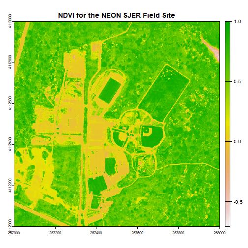
ndviCalc <- app(ndviStack,NDVI)
plot(ndviCalc, main="NDVI for the NEON SJER Field Site")
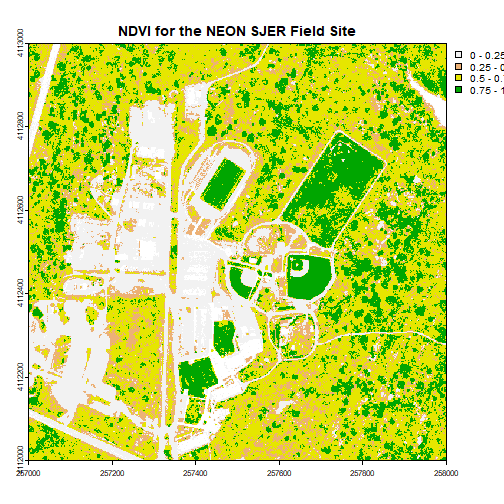
# Now, play with breaks and colors to create a meaningful map
# add a color map with 4 colors

myCol <- rev(terrain.colors(4)) # use the 'rev()' function to put green as the highest NDVI value
# add breaks to the colormap, including lowest and highest values (4 breaks = 3 segments)

brk <- c(0, .25, .5, .75, 1)

# plot the image using breaks
plot(ndviCalc, main="NDVI for the NEON SJER Field Site", col=myCol, breaks=brk)
Challenge: Work with Indices
Try the following on your own:
- Calculate the Normalized Difference Nitrogen Index (NDNI) using the following equation:
$$ NDNI = \frac{log(\frac{1}{p_{1510}}) - log(\frac{1}{p_{1680}})}{log(\frac{1}{p_{1510}}) + log(\frac{1}{p_{1680}})} $$ 2. Calculate the Enhanced Vegetation Index (EVI). Hint: Look up the formula, and apply the appropriate NEON bands. Hint: You can look at satellite datasets, such as USGS Landsat EVI.
- Explore the bands in the hyperspectral data. What happens if you average reflectance values across multiple Red and NIR bands and then calculate NDVI?