Going On The Grid -- An Intro to Gridding & Spatial Interpolation

In this tutorial was originally created for an ESA brown-bag workshop. Here we present the main graphics and topics covered in the workshop.

How Does LiDAR Works?

About Rasters

For a full tutorial on rasters & raster data, please go through the Intro to Raster Data in R tutorial which provides a foundational concepts even if you aren't working with R.

A raster is a dataset made up of cells or pixels. Each pixel represents a value associated with a region on the earth’s surface.

For more on raster resolution, see our tutorial on The Relationship Between Raster Resolution, Spatial Extent & Number of Pixels.

Creating Surfaces (Rasters) From Points

There are several ways that we can get from the point data collected by lidar to the surface data that we want for different Digital Elevation Models or similar data we use in analyses and mapping.

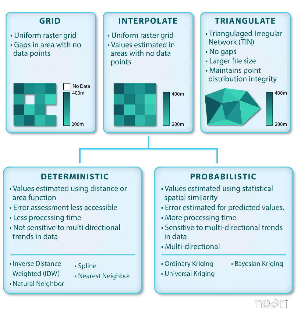
Basic gridding does not allow for the recovery/classification of data in any area where data are missing. Interpolation (including Triangulated Irregular Network (TIN) Interpolation) allows for gaps to be covered so that there are not holes in the resulting raster surface.

Interpolation can be done in a number of different ways, some of which are deterministic and some are probabilistic.

Gridding Points

When creating a raster, you may chose to perform a direct gridding of the data. This means that you calculate one value for every cell in the raster where there are sample points. This value may be a mean of all points, a max, min or some other mathematical function. All other cells will then have no data values associated with them. This means you may have gaps in your data if the point spacing is not well distributed with at least one data point within the spatial coverage of each raster cell.

We can create a raster from points through a process called gridding. Gridding is the process of taking a set of points and using them to create a surface composed of a regular grid.

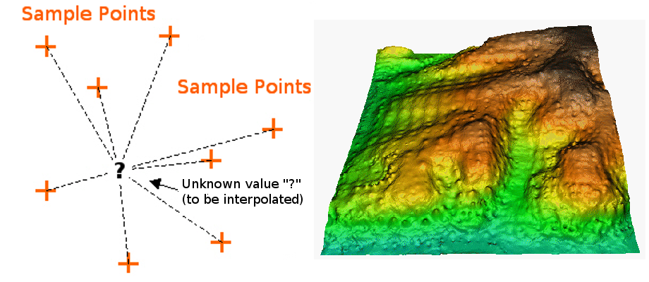
Spatial Interpolation

Spatial interpolation involves calculating the value for a query point (or a raster cell) with an unknown value from a set of known sample point values that are distributed across an area. There is a general assumption that points closer to the query point are more strongly related to that cell than those farther away. However this general assumption is applied differently across different interpolation functions.

Deterministic & Probabilistic Interpolators

There are two main types of interpolation approaches:

• Deterministic: create surfaces directly from measured points using a weighted distance or area function.
• Probabilistic (Geostatistical): utilize the statistical properties of the measured points. Probabilistic techniques quantify the spatial auto-correlation among measured points and account for the spatial configuration of the sample points around the prediction location.

Different methods of interpolation are better for different datasets. This table lays out the strengths of some of the more common interpolation methods.

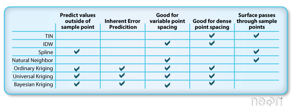
We will focus on deterministic methods in this tutorial.

Deterministic Interpolation Methods

Let's look at a few different deterministic interpolation methods to understand how different methods can affect an output raster.

Inverse Distance Weighted (IDW)

Inverse distance weighted (IDW) interpolation calculates the values of a query point (a cell with an unknown value) using a linearly weighted combination of values from nearby points.

Key Attributes of IDW Interpolation

• The raster is derived based upon an assumed linear relationship between the location of interest and the distance to surrounding sample points. In other words, sample points closest to the cell of interest are assumed to be more related to its value than those further away.ID
• Bounded/exact estimation, hence can not interpolate beyond the min/max range of data point values. This estimate within the range of existing sample point values can yield "flattened" peaks and valleys -- especially if the data didn't capture those high and low points.
• Interpolated points are average values
• Good for point data that are equally distributed and dense. Assumes a consistent trend or relationship between points and does not accommodate trends within the data(e.g. east to west, elevational, etc).

Power

The power value changes the "weighting" of the IDW interpolation by specifying how strongly points further away from the query point impact the calculated value for that point. Power values range from 0-3+ with a default settings generally being 2. A larger power value produces a more localized result - values further away from the cell have less impact on it's calculated value, values closer to the cell impact it's value more. A smaller power value produces a more averaged result where sample points further away from the cell have a greater impact on the cell's calculated value.

For visualizations of IDW interpolation, see Jochen Albrecht's Inverse Distance Weighted 3D Concepts Lecture.

The impacts of power:

• lower power values more averaged result, potential for a smoother surface. As power decreases, the influence of sample points is larger. This yields a smoother surface that is more averaged.

• greater power values: more localized result, potential for more peaks and valleys around sample point locations. As power increases, the influence of sample points falls off more rapidly with distance. The query cell values become more localized and less averaged.

IDW Take Home Points

IDW is good for:

• Data whose distribution is strongly (and linearly) correlated with distance. For example, noise falls off very predictably with distance.
• Providing explicit control over the influence of distance (compared to Spline or Kriging).

IDW is not so good for:

• Data whose distribution depends on more complex sets of variables because it can account only for the effects of distance.

Other features:

• You can create a smoother surface by decreasing the power, increasing the number of sample points used or increasing the search (sample points) radius.
• You can create a surface that more closely represents the peaks and dips of your sample points by decreasing the number of sample points used, decreasing the search radius or increasing the power.
• You can increase IDW surface accuracy by adding breaklines to the interpolation process that serve as barriers. Breaklines represent abrupt changes in elevation, such as cliffs.

Spline

Spline interpolation fits a curved surface through the sample points of your dataset. Imagine stretching a rubber sheet across your points and gluing it to each sample point along the way -- what you get is a smooth stretched sheet with bumps and valleys. Unlike IDW, spline can estimate values above and below the min and max values of your sample points. Thus it is good for estimating high and low values not already represented in your data.

For visualizations of Spline interpolation, see Jochen Albrecht's Spline 3D Concepts Lecture.

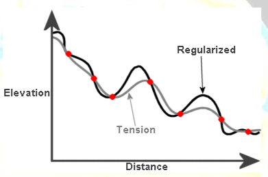
Regularized & Tension Spline

There are two types of curved surfaces that can be fit when using spline interpolation:

1. Tension spline: a flatter surface that forces estimated values to stay closer to the known sample points.

2. Regularized spline: a more elastic surface that is more likely to estimate above and below the known sample points.

For more on spline interpolation, see ESRI's How Splines Work background materials.

Spline Take Home Points

Spline is good for:

• Estimating values outside of the range of sample input data.
• Creating a smooth continuous surface.

Spline is not so good for:

• Points that are close together and have large value differences. Slope calculations can yield over and underestimation.
• Data with large, sudden changes in values that need to be represented (e.g., fault lines, extreme vertical topographic changes, etc). NOTE: some tools like ArcGIS have introduced a spline with barriers function in recent years.

Natural Neighbor Interpolation

Natural neighbor interpolation finds the closest subset of data points to the query point of interest. It then applies weights to those points to calculate an average estimated value based upon their proportionate areas derived from their corresponding Voronoi polygons (see figure below for definition). The natural neighbor interpolator adapts locally to the input data using points surrounding the query point of interest. Thus there is no radius, number of points or other settings needed when using this approach.

This interpolation method works equally well on regular and irregularly spaced data.

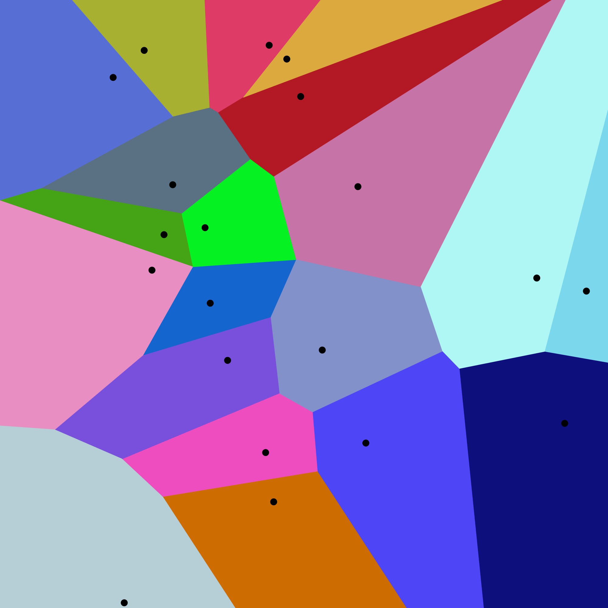
Natural neighbor interpolation uses the area of each Voronoi polygon associated with the surrounding points to derive a weight that is then used to calculate an estimated value for the query point of interest.

To calculate the weighted area around a query point, a secondary Voronoi diagram is created using the immediately neighboring points and mapped on top of the original Voronoi diagram created using the known sample points (image below).

For more on natural neighbor interpolation, see ESRI's How Natural Neighbor Works documentation.

Natural Neighbor Take Home Points

Natural Neighbor Interpolation is good for:

• Data where spatial distribution is variable (and data that are equally distributed).
• Categorical data.
• Providing a smoother output raster.

Natural Neighbor Interpolation is not as good for:

• Data where the interpolation needs to be spatially constrained (to a particular number of points of distance).
• Data where sample points further away from or beyond the immediate "neighbor points" need to be considered in the estimation.

Other features:

• Good as a local interpolator
• Interpolated values fall within the range of values of the sample data
• Surface passes through input samples; not above or below
• Supports breaklines

Triangulated Irregular Network (TIN)

The Triangulated Irregular Network (TIN) is a vector based surface where sample points (nodes) are connected by a series of edges creating a triangulated surface. The TIN format remains the most true to the point distribution, density and spacing of a dataset. It also may yield the largest file size!

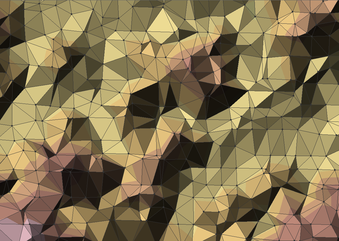
• For more on the TIN process see this information from ESRI: Overview of TINs

Interpolation in R, GrassGIS, or QGIS

These additional resources point to tools and information for gridding in R, GRASS GIS and QGIS.

R functions

The packages and functions maybe useful when creating grids in R.

• gstat::idw()
• stats::loess()
• akima::interp()
• fields::Tps()
• fields::splint()
• spatial::surf.ls()
• geospt::rbf()

QGIS tools

• Check out the documentation on different interpolation plugins Interpolation
• Check out the documentation on how to convert a vector file to a raster: Rasterize (vector to raster).

The QGIS processing toolbox provides easy access to Grass commands.

GrassGIS commands

• Check out the documentation on GRASS GIS Integration Starting the GRASS plugin

The following commands may be useful if you are working with GrassGIS.

• v.surf.idw - Surface interpolation from vector point data by Inverse Distance Squared Weighting
• v.surf.bspline - Bicubic or bilinear spline interpolation with Tykhonov regularization
• v.surf.rst - Spatial approximation and topographic analysis using regularized spline with tension
• v.to.rast.value - Converts (rasterize) a vector layer into a raster layer
• v.delaunay - Creates a Delaunay triangulation from an input vector map containing points or centroids
• v.voronoi - Creates a Voronoi diagram from an input vector layer containing points