Tutorial
Using the NEON API in R
Last Updated: Apr 2, 2026
This is a tutorial in pulling data from the NEON API or Application Programming Interface. The tutorial uses R and the R package httr, but the core information about the API is applicable to other languages and approaches.
Objectives
After completing this activity, you will be able to:
- Construct API calls to query the NEON API.
- Access and understand data and metadata available via the NEON API.
Things You’ll Need To Complete This Tutorial
To complete this tutorial you will need the most current version of R and, preferably, RStudio loaded on your computer.
Install R Packages
-
httr:
install.packages("httr") -
jsonlite:
install.packages("jsonlite")
Additional Resources
What is an API?
If you are unfamiliar with the concept of an API, think of an API as a ‘middle person' that provides a communication path for a software application to obtain information from a digital data source. APIs are becoming a very common means of sharing digital information. Many of the apps that you use on your computer or mobile device to produce maps, charts, reports, and other useful forms of information pull data from multiple sources using APIs. In the ecological and environmental sciences, many researchers use APIs to programmatically pull data into their analyses. (Quoted from the NEON Observatory Blog story: API and data availability viewer now live on the NEON data portal.)
What is accessible via the NEON API?
The NEON API includes endpoints for NEON data and metadata, including spatial data, taxonomic data, and samples (see Endpoints below). This tutorial explores these sources of information using a specific data product as a guide. The principles and rule sets described below can be applied to other data products and metadata.
Anatomy of an API call
An example API call: http://data.neonscience.org/api/v0/data/DP1.10003.001/WOOD/2015-07
This includes the base URL, endpoint, and target.
Base URL:
http://data.neonscience.org/api/v0/data/DP1.10003.001/WOOD/2015-07
Specifics are appended to this in order to get the data or metadata you're looking for, but all calls to an API will include the base URL. For the NEON API, this is http://data.neonscience.org/api/v0 -- not clickable, because the base URL by itself will take you nowhere!
Endpoints:
http://data.neonscience.org/api/v0/data/DP1.10098.001/WOOD/2015-07
What type of data or metadata are you looking for?
-
~/products Information about one or all of NEON's data products
-
~/sites Information about data availability at the site specified in the call
-
~/locations Spatial data for the NEON locations specified in the call
-
~/data Data! By product, site, and date (in monthly chunks)
-
~/samples Information about sample relationships and sample tracking
-
~/taxonomy Access to NEON's taxon lists, the approved scientific names for sampled taxa
Targets:
http://data.neonscience.org/api/v0/data/DP1.10098.001/WOOD/2015-07
The specific data product, location, sample, etc, you want to get data for.
Data, by way of Products
Which product do you want to get data for? Consult the Explore Data Products page.
We'll pick Woody vegetation structure, DP1.10098.001
Your first thought is probably to use the /data endpoint. And we'll get there. But notice above that the API call for the /data endpoint includes the site and month of data to download. You don't want to have to guess sites and months at random - first, you need to see which sites and months have available data for the product you're interested in. That can be done either through the /sites or the /products endpoint; here we'll use /products.
Note: Checking for data availability can sometimes be skipped for the streaming sensor data products. In general, they are available continuously, and you could theoretically query a site and month of interest and expect there to be data by default. However, there can be interruptions to sensor data, in particular at aquatic sites, so checking availability first is the most reliable approach.
Use the products endpoint to query for Woody vegetation data. The target is the data product identifier, noted above, DP1.10098.001:
# Load the necessary libraries
library(httr)
library(jsonlite)

# Request data using the GET function & the API call
req <- GET("http://data.neonscience.org/api/v0/products/DP1.10098.001")
req

## Response [https://data.neonscience.org/api/v0/products/DP1.10098.001]
##   Date: 2021-06-16 01:03
##   Status: 200
##   Content-Type: application/json;charset=UTF-8
##   Size: 70.1 kB
The object returned from GET() has many layers of information. Entering the
name of the object gives you some basic information about what you accessed.
Status: 200 indicates this was a successful query; the status field can be
a useful place to look if something goes wrong. These are HTTP status codes,
you can google them to find out what a given value indicates.
The Content-Type parameter tells us we've accessed a json file. The easiest
way to translate this to something more manageable in R is to use the
fromJSON() function in the jsonlite package. It will convert the json into
a nested list, flattening the nesting where possible.
# Make the data readable by jsonlite
req.text <- content(req, as="text")

# Flatten json into a nested list
avail <- jsonlite::fromJSON(req.text,
                            simplifyDataFrame=T,
                            flatten=T)
A lot of the content here is basic information about the data product.
You can see all of it by running the line print(avail), but
this will result in a very long printout in your console. Instead, try viewing
list items individually. Here, we highlight a couple of interesting examples:
# View description of data product
avail$data$productDescription

## [1] "Structure measurements, including height, crown diameter, and stem diameter, as well as mapped position of individual woody plants"

# View data product abstract
avail$data$productAbstract

## [1] "This data product contains the quality-controlled, native sampling resolution data from in-situ measurements of live and standing dead woody individuals and shrub groups, from all terrestrial NEON sites with qualifying woody vegetation. The exact measurements collected per individual depend on growth form, and these measurements are focused on enabling biomass and productivity estimation, estimation of shrub volume and biomass, and calibration / validation of multiple NEON airborne remote-sensing data products. In general, comparatively large individuals that are visible to remote-sensing instruments are mapped, tagged and measured, and other smaller individuals are tagged and measured but not mapped. Smaller individuals may be subsampled according to a nested subplot approach in order to standardize the per plot sampling effort. Structure and mapping data are reported per individual per plot; sampling metadata, such as per growth form sampling area, are reported per plot. For additional details, see the user guide, protocols, and science design listed in the Documentation section in this data product's details webpage.\n\nLatency:\nThe expected time from data and/or sample collection in the field to data publication is as follows, for each of the data tables (in days) in the downloaded data package. See the Data Product User Guide for more information.\n\nvst_apparentindividual:  90\n\nvst_mappingandtagging:  90\n\nvst_perplotperyear:  300\n\nvst_shrubgroup:  90"
You may notice that some of this information is also accessible on the NEON data portal. The portal uses the same data sources as the API, and in many cases the portal is using the API on the back end, and simply adding a more user-friendly display to the data.
We want to find which sites and months have available data. That is in the
siteCodes section. Let's look at what information is presented for each
site:
# Look at the first list element for siteCode
avail$data$siteCodes$siteCode[[1]]

## [1] "ABBY"

# And at the first list element for availableMonths
avail$data$siteCodes$availableMonths[[1]]

##  [1] "2015-07" "2015-08" "2016-08" "2016-09" "2016-10" "2016-11" "2017-03" "2017-04" "2017-07" "2017-08"
## [11] "2017-09" "2018-07" "2018-08" "2018-09" "2018-10" "2018-11" "2019-07" "2019-09" "2019-10" "2019-11"
Here we can see the list of months with data for the site ABBY, which is the Abby Road forest in Washington state.
The section $data$siteCodes$availableDataUrls provides the exact API
calls we need in order to query the data for each available site and month.
# Get complete list of available data URLs
wood.urls <- unlist(avail$data$siteCodes$availableDataUrls)

# Total number of URLs
length(wood.urls)

## [1] 535

# Show first 10 URLs available
wood.urls[1:10]

##  [1] "https://data.neonscience.org/api/v0/data/DP1.10098.001/ABBY/2015-07"
##  [2] "https://data.neonscience.org/api/v0/data/DP1.10098.001/ABBY/2015-08"
##  [3] "https://data.neonscience.org/api/v0/data/DP1.10098.001/ABBY/2016-08"
##  [4] "https://data.neonscience.org/api/v0/data/DP1.10098.001/ABBY/2016-09"
##  [5] "https://data.neonscience.org/api/v0/data/DP1.10098.001/ABBY/2016-10"
##  [6] "https://data.neonscience.org/api/v0/data/DP1.10098.001/ABBY/2016-11"
##  [7] "https://data.neonscience.org/api/v0/data/DP1.10098.001/ABBY/2017-03"
##  [8] "https://data.neonscience.org/api/v0/data/DP1.10098.001/ABBY/2017-04"
##  [9] "https://data.neonscience.org/api/v0/data/DP1.10098.001/ABBY/2017-07"
## [10] "https://data.neonscience.org/api/v0/data/DP1.10098.001/ABBY/2017-08"
These URLs are the API calls we can use to find out what files are available for each month where there are data. They are pre-constructed calls to the /data endpoint of the NEON API.
Let's look at the woody plant data from the Rocky Mountain National Park
(RMNP) site from October 2019. We can do this by using the GET() function
on the relevant URL, which we can extract using the grep() function.
Note that if you want data from more than one site/month you need to iterate
this code, GET() fails if you give it more than one URL at a time.
# Get available data for RMNP Oct 2019
woody <- GET(wood.urls[grep("RMNP/2019-10", wood.urls)])
woody.files <- jsonlite::fromJSON(content(woody, as="text"))

# See what files are available for this site and month
woody.files$data$files$name

## [1] "NEON.D10.RMNP.DP1.10098.001.EML.20191010-20191017.20210123T023002Z.xml"
## [2] "NEON.D10.RMNP.DP1.10098.001.2019-10.basic.20210114T173951Z.zip"
## [3] "NEON.D10.RMNP.DP1.10098.001.vst_apparentindividual.2019-10.basic.20210114T173951Z.csv"
## [4] "NEON.D10.RMNP.DP1.10098.001.variables.20210114T173951Z.csv"
## [5] "NEON.D10.RMNP.DP0.10098.001.categoricalCodes.20210114T173951Z.csv"
## [6] "NEON.D10.RMNP.DP1.10098.001.readme.20210123T023002Z.txt"
## [7] "NEON.D10.RMNP.DP1.10098.001.vst_perplotperyear.2019-10.basic.20210114T173951Z.csv"
## [8] "NEON.D10.RMNP.DP1.10098.001.vst_mappingandtagging.basic.20210114T173951Z.csv"
## [9] "NEON.D10.RMNP.DP0.10098.001.validation.20210114T173951Z.csv"
If you've downloaded NEON data before via the data portal or the
neonUtilities package, this should look very familiar. The format
for most of the file names is:
NEON.[domain number].[site code].[data product ID].[file-specific name]. [year and month of data].[basic or expanded data package]. [date of file creation]
Some files omit the year and month, and/or the data package, since they're not specific to a particular measurement interval, such as the data product readme and variables files. The date of file creation uses the ISO6801 format, for example 20210114T173951Z, and can be used to determine whether data have been updated since the last time you downloaded.
Available files in our query for October 2019 at Rocky Mountain are all of the following (leaving off the initial NEON.D10.RMNP.DP1.10098.001):
-
~.vst_perplotperyear.2019-10.basic.20210114T173951Z.csv: data table of measurements conducted at the plot level every year
-
~.vst_apparentindividual.2019-10.basic.20210114T173951Z.csv: data table containing measurements and observations conducted on woody individuals
-
~.vst_mappingandtagging.basic.20210114T173951Z.csv: data table containing mapping data for each measured woody individual. Note year and month are not in file name; these data are collected once per individual and provided with every month of data downloaded
-
~.categoricalCodes.20210114T173951Z.csv: definitions of the values in categorical variables
-
~.readme.20210123T023002Z.txt: readme for the data product (not specific to dates or location)
-
~.EML.20191010-20191017.20210123T023002Z.xml: Ecological Metadata Language (EML) file, describing the data product
-
~.validation.20210114T173951Z.csv: validation file for the data product, lists input data and data entry validation rules
-
~.variables.20210114T173951Z.csv: variables file for the data product, lists data fields in downloaded tables
-
~.2019-10.basic.20210114T173951Z.zip: zip of all files in the basic package. Pre-packaged zips are planned to be removed; may not appear in response to your query
This data product doesn't have an expanded package, so we only see the basic package data files, and only one copy of each of the metadata files.
Let's get the data table for the mapping and tagging data. The list of files doesn't return in the same order every time, so we shouldn't use the position in the list to select the file name we want. Plus, we want code we can re-use when getting data from other sites and other months. So we select file urls based on the data table name in the file names.
vst.maptag <- read.csv(woody.files$data$files$url
                       [grep("mappingandtagging",
                             woody.files$data$files$name)])
Note that if there were an expanded package, the code above would return two URLs. In that case you would need to specify the package as well in selecting the URL.
Now we have the data and can access it in R. Just to show that the file we pulled has actual data in it, let's make a quick graphic of the species present and their abundances:
# Get counts by species
countBySp <- table(vst.maptag$taxonID)

# Reorder so list is ordered most to least abundance
countBySp <- countBySp[order(countBySp, decreasing=T)]

# Plot abundances
barplot(countBySp, names.arg=names(countBySp),
        ylab="Total", las=2)
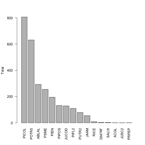
This shows us that the two most abundant species are designated with the taxon codes PICOL and POTR5. We can look back at the data table, check the scientificName field corresponding to these values, and see that these are lodgepole pine and quaking aspen, as we might expect in the eastern foothills of the Rocky mountains.
Let's say we're interested in how NEON defines quaking aspen, and what taxon authority it uses for its definition. We can use the /taxonomy endpoint of the API to do that.
Taxonomy
NEON maintains accepted taxonomies for many of the taxonomic identification data we collect. NEON taxonomies are available for query via the API; they are also provided via an interactive user interface, the Taxon Viewer.
NEON taxonomy data provides the reference information for how NEON validates taxa; an identification must appear in the taxonomy lists in order to be accepted into the NEON database. Additions to the lists are reviewed regularly. The taxonomy lists also provide the author of the scientific name, and the reference text used.
The taxonomy endpoint of the API has query options that are a bit more complicated than what was described in the "Anatomy of an API Call" section above. As described above, each endpoint has a single type of target - a data product number, a named location name, etc. For taxonomic data, there are multiple query options, and some of them can be used in combination. Instead of entering a single target, we specify the query type, and then the query parameter to search for. For example, a query for taxa in the Pinaceae family:
http://data.neonscience.org/api/v0/taxonomy/?family=Pinaceae
The available types of queries are listed in the taxonomy section of the API web page. Briefly, they are:
-
taxonTypeCode: Which of the taxonomies maintained by NEON are you looking for? BIRD, FISH, PLANT, etc. Cannot be used in combination with the taxonomic rank queries. - each of the major taxonomic ranks from genus through kingdom
-
scientificname: Genus + specific epithet (+ authority). Search is by exact match only, see final example below. -
verbose: Do you want the short (false) or long (true) response -
offset: Skip this number of items at the start of the list. -
limit: Result set will be truncated at this length.
For the first example, let's query for the loon family, Gaviidae, in the bird taxonomy. Note that query parameters are case-sensitive.
loon.req <- GET("http://data.neonscience.org/api/v0/taxonomy/?family=Gaviidae")
Parse the results into a list using fromJSON():
loon.list <- jsonlite::fromJSON(content(loon.req, as="text"))
And look at the $data element of the results, which contains:
- The full taxonomy of each taxon
- The short taxon code used by NEON (taxonID/acceptedTaxonID)
- The author of the scientific name (scientificNameAuthorship)
- The vernacular name, if applicable
- The reference text used (nameAccordingToID)
The terms used for each field are matched to Darwin Core (dwc) and the Global Biodiversity Information Facility (gbif) terms, where possible, and the matches are indicated in the column headers.
loon.list$data

##   taxonTypeCode taxonID acceptedTaxonID dwc:scientificName dwc:scientificNameAuthorship dwc:taxonRank
## 1          BIRD    ARLO            ARLO      Gavia arctica                   (Linnaeus)       species
## 2          BIRD    COLO            COLO        Gavia immer                   (Brunnich)       species
## 3          BIRD    PALO            PALO     Gavia pacifica                   (Lawrence)       species
## 4          BIRD    RTLO            RTLO     Gavia stellata                (Pontoppidan)       species
## 5          BIRD    YBLO            YBLO      Gavia adamsii                 (G. R. Gray)       species
##   dwc:vernacularName    dwc:nameAccordingToID dwc:kingdom dwc:phylum dwc:class   dwc:order dwc:family
## 1        Arctic Loon doi: 10.1642/AUK-15-73.1    Animalia   Chordata      Aves Gaviiformes   Gaviidae
## 2        Common Loon doi: 10.1642/AUK-15-73.1    Animalia   Chordata      Aves Gaviiformes   Gaviidae
## 3       Pacific Loon doi: 10.1642/AUK-15-73.1    Animalia   Chordata      Aves Gaviiformes   Gaviidae
## 4  Red-throated Loon doi: 10.1642/AUK-15-73.1    Animalia   Chordata      Aves Gaviiformes   Gaviidae
## 5 Yellow-billed Loon doi: 10.1642/AUK-15-73.1    Animalia   Chordata      Aves Gaviiformes   Gaviidae
##   dwc:genus gbif:subspecies gbif:variety
## 1     Gavia              NA           NA
## 2     Gavia              NA           NA
## 3     Gavia              NA           NA
## 4     Gavia              NA           NA
## 5     Gavia              NA           NA
To get the entire list for a particular taxonomic type, use the
taxonTypeCode query. Be cautious with this query, the PLANT taxonomic
list has several hundred thousand entries.
For an example, let's look up the small mammal taxonomic list, which
is one of the shorter ones, and use the verbose=true option to see
a more extensive list of taxon data, including many taxon ranks that
aren't populated for these taxa. For space here, we'll display only
the first 10 taxa:
mam.req <- GET("http://data.neonscience.org/api/v0/taxonomy/?taxonTypeCode=SMALL_MAMMAL&verbose=true")
mam.list <- jsonlite::fromJSON(content(mam.req, as="text"))
mam.list$data[1:10,]

##    taxonTypeCode taxonID acceptedTaxonID               dwc:scientificName dwc:scientificNameAuthorship
## 1   SMALL_MAMMAL    AMHA            AMHA        Ammospermophilus harrisii          Audubon and Bachman
## 2   SMALL_MAMMAL    AMIN            AMIN       Ammospermophilus interpres                      Merriam
## 3   SMALL_MAMMAL    AMLE            AMLE        Ammospermophilus leucurus                      Merriam
## 4   SMALL_MAMMAL    AMLT            AMLT Ammospermophilus leucurus tersus                      Goldman
## 5   SMALL_MAMMAL    AMNE            AMNE         Ammospermophilus nelsoni                      Merriam
## 6   SMALL_MAMMAL    AMSP            AMSP             Ammospermophilus sp.                         <NA>
## 7   SMALL_MAMMAL    APRN            APRN            Aplodontia rufa nigra                       Taylor
## 8   SMALL_MAMMAL    APRU            APRU                  Aplodontia rufa                   Rafinesque
## 9   SMALL_MAMMAL    ARAL            ARAL                Arborimus albipes                      Merriam
## 10  SMALL_MAMMAL    ARLO            ARLO            Arborimus longicaudus                         True
##    dwc:taxonRank            dwc:vernacularName taxonProtocolCategory dwc:nameAccordingToID
## 1        species     Harriss Antelope Squirrel         opportunistic  isbn: 978 0801882210
## 2        species       Texas Antelope Squirrel         opportunistic  isbn: 978 0801882210
## 3        species Whitetailed Antelope Squirrel         opportunistic  isbn: 978 0801882210
## 4     subspecies                          <NA>         opportunistic  isbn: 978 0801882210
## 5        species     Nelsons Antelope Squirrel         opportunistic  isbn: 978 0801882210
## 6          genus                          <NA>         opportunistic  isbn: 978 0801882210
## 7     subspecies                          <NA>            non-target  isbn: 978 0801882210
## 8        species                      Sewellel            non-target  isbn: 978 0801882210
## 9        species              Whitefooted Vole                target  isbn: 978 0801882210
## 10       species                 Red Tree Vole                target  isbn: 978 0801882210
##                                                                                                                                                 dwc:nameAccordingToTitle
## 1  Wilson D. E. and D. M. Reeder. 2005. Mammal Species of the World; A Taxonomic and Geographic Reference. Third edition. Johns Hopkins University Press; Baltimore, MD.
## 2  Wilson D. E. and D. M. Reeder. 2005. Mammal Species of the World; A Taxonomic and Geographic Reference. Third edition. Johns Hopkins University Press; Baltimore, MD.
## 3  Wilson D. E. and D. M. Reeder. 2005. Mammal Species of the World; A Taxonomic and Geographic Reference. Third edition. Johns Hopkins University Press; Baltimore, MD.
## 4  Wilson D. E. and D. M. Reeder. 2005. Mammal Species of the World; A Taxonomic and Geographic Reference. Third edition. Johns Hopkins University Press; Baltimore, MD.
## 5  Wilson D. E. and D. M. Reeder. 2005. Mammal Species of the World; A Taxonomic and Geographic Reference. Third edition. Johns Hopkins University Press; Baltimore, MD.
## 6  Wilson D. E. and D. M. Reeder. 2005. Mammal Species of the World; A Taxonomic and Geographic Reference. Third edition. Johns Hopkins University Press; Baltimore, MD.
## 7  Wilson D. E. and D. M. Reeder. 2005. Mammal Species of the World; A Taxonomic and Geographic Reference. Third edition. Johns Hopkins University Press; Baltimore, MD.
## 8  Wilson D. E. and D. M. Reeder. 2005. Mammal Species of the World; A Taxonomic and Geographic Reference. Third edition. Johns Hopkins University Press; Baltimore, MD.
## 9  Wilson D. E. and D. M. Reeder. 2005. Mammal Species of the World; A Taxonomic and Geographic Reference. Third edition. Johns Hopkins University Press; Baltimore, MD.
## 10 Wilson D. E. and D. M. Reeder. 2005. Mammal Species of the World; A Taxonomic and Geographic Reference. Third edition. Johns Hopkins University Press; Baltimore, MD.
##    dwc:kingdom gbif:subkingdom gbif:infrakingdom gbif:superdivision gbif:division gbif:subdivision
## 1     Animalia              NA                NA                 NA            NA               NA
## 2     Animalia              NA                NA                 NA            NA               NA
## 3     Animalia              NA                NA                 NA            NA               NA
## 4     Animalia              NA                NA                 NA            NA               NA
## 5     Animalia              NA                NA                 NA            NA               NA
## 6     Animalia              NA                NA                 NA            NA               NA
## 7     Animalia              NA                NA                 NA            NA               NA
## 8     Animalia              NA                NA                 NA            NA               NA
## 9     Animalia              NA                NA                 NA            NA               NA
## 10    Animalia              NA                NA                 NA            NA               NA
##    gbif:infradivision gbif:parvdivision gbif:superphylum dwc:phylum gbif:subphylum gbif:infraphylum
## 1                  NA                NA               NA   Chordata             NA               NA
## 2                  NA                NA               NA   Chordata             NA               NA
## 3                  NA                NA               NA   Chordata             NA               NA
## 4                  NA                NA               NA   Chordata             NA               NA
## 5                  NA                NA               NA   Chordata             NA               NA
## 6                  NA                NA               NA   Chordata             NA               NA
## 7                  NA                NA               NA   Chordata             NA               NA
## 8                  NA                NA               NA   Chordata             NA               NA
## 9                  NA                NA               NA   Chordata             NA               NA
## 10                 NA                NA               NA   Chordata             NA               NA
##    gbif:superclass dwc:class gbif:subclass gbif:infraclass gbif:superorder dwc:order gbif:suborder
## 1               NA  Mammalia            NA              NA              NA  Rodentia            NA
## 2               NA  Mammalia            NA              NA              NA  Rodentia            NA
## 3               NA  Mammalia            NA              NA              NA  Rodentia            NA
## 4               NA  Mammalia            NA              NA              NA  Rodentia            NA
## 5               NA  Mammalia            NA              NA              NA  Rodentia            NA
## 6               NA  Mammalia            NA              NA              NA  Rodentia            NA
## 7               NA  Mammalia            NA              NA              NA  Rodentia            NA
## 8               NA  Mammalia            NA              NA              NA  Rodentia            NA
## 9               NA  Mammalia            NA              NA              NA  Rodentia            NA
## 10              NA  Mammalia            NA              NA              NA  Rodentia            NA
##    gbif:infraorder gbif:section gbif:subsection gbif:superfamily    dwc:family gbif:subfamily gbif:tribe
## 1               NA           NA              NA               NA     Sciuridae        Xerinae  Marmotini
## 2               NA           NA              NA               NA     Sciuridae        Xerinae  Marmotini
## 3               NA           NA              NA               NA     Sciuridae        Xerinae  Marmotini
## 4               NA           NA              NA               NA     Sciuridae        Xerinae  Marmotini
## 5               NA           NA              NA               NA     Sciuridae        Xerinae  Marmotini
## 6               NA           NA              NA               NA     Sciuridae        Xerinae  Marmotini
## 7               NA           NA              NA               NA Aplodontiidae           <NA>       <NA>
## 8               NA           NA              NA               NA Aplodontiidae           <NA>       <NA>
## 9               NA           NA              NA               NA    Cricetidae    Arvicolinae       <NA>
## 10              NA           NA              NA               NA    Cricetidae    Arvicolinae       <NA>
##    gbif:subtribe        dwc:genus dwc:subgenus gbif:subspecies gbif:variety gbif:subvariety gbif:form
## 1             NA Ammospermophilus         <NA>              NA           NA              NA        NA
## 2             NA Ammospermophilus         <NA>              NA           NA              NA        NA
## 3             NA Ammospermophilus         <NA>              NA           NA              NA        NA
## 4             NA Ammospermophilus         <NA>              NA           NA              NA        NA
## 5             NA Ammospermophilus         <NA>              NA           NA              NA        NA
## 6             NA Ammospermophilus         <NA>              NA           NA              NA        NA
## 7             NA       Aplodontia         <NA>              NA           NA              NA        NA
## 8             NA       Aplodontia         <NA>              NA           NA              NA        NA
## 9             NA        Arborimus         <NA>              NA           NA              NA        NA
## 10            NA        Arborimus         <NA>              NA           NA              NA        NA
##    gbif:subform speciesGroup dwc:specificEpithet dwc:infraspecificEpithet
## 1            NA         <NA>            harrisii                     <NA>
## 2            NA         <NA>           interpres                     <NA>
## 3            NA         <NA>            leucurus                     <NA>
## 4            NA         <NA>            leucurus                   tersus
## 5            NA         <NA>             nelsoni                     <NA>
## 6            NA         <NA>                 sp.                     <NA>
## 7            NA         <NA>                rufa                    nigra
## 8            NA         <NA>                rufa                     <NA>
## 9            NA         <NA>             albipes                     <NA>
## 10           NA         <NA>         longicaudus                     <NA>
Now let's go back to our question about quaking aspen. To get
information about a single taxon, use the scientificname
query. This query will not do a fuzzy match, so you need to query
the exact name of the taxon in the NEON taxonomy. Because of this,
the query will be most useful in cases like the current one, where
you already have NEON data in hand and are looking for more
information about a specific taxon. Querying on scientificname
is unlikely to be an efficient way to figure out if NEON recognizes
a particular taxon.
In addition, scientific names contain spaces, which are not allowed in a URL. The spaces need to be replaced with the URL encoding replacement, %20.
Looking up the POTR5 data in the woody vegetation product, we
see that the scientific name is Populus tremuloides Michx.
This means we need to search for Populus%20tremuloides%20Michx.
to get the exact match.
aspen.req <- GET("http://data.neonscience.org/api/v0/taxonomy/?scientificname=Populus%20tremuloides%20Michx.")
aspen.list <- jsonlite::fromJSON(content(aspen.req, as="text"))
aspen.list$data

##   taxonTypeCode taxonID acceptedTaxonID         dwc:scientificName dwc:scientificNameAuthorship
## 1         PLANT   POTR5           POTR5 Populus tremuloides Michx.                       Michx.
##   dwc:taxonRank dwc:vernacularName                       dwc:nameAccordingToID dwc:kingdom    dwc:phylum
## 1       species      quaking aspen http://plants.usda.gov (accessed 8/25/2014)     Plantae Magnoliophyta
##       dwc:class dwc:order dwc:family dwc:genus gbif:subspecies gbif:variety
## 1 Magnoliopsida Salicales Salicaceae   Populus              NA           NA
This shows us the definition for Populus tremuloides Michx. does
not include a subspecies or variety, and the authority for the
taxon information (nameAccordingToID) is the USDA PLANTS
database. This means NEON taxonomic definitions are aligned with
the USDA, and is true for the large majority of plants in the
NEON taxon system.
Spatial data
How to get spatial data and what to do with it depends on which type of data you're working with.
Instrumentation data (both aquatic and terrestrial)
The sensor_positions files, which are included in the list of available files, contain spatial coordinates for each sensor in the data. See the final section of the Geolocation tutorial for guidance in using these files.
Observational data - Aquatic
Latitude, longitude, elevation, and associated uncertainties are included in data downloads. Most products also include an "additional coordinate uncertainty" that should be added to the provided uncertainty. Additional spatial data, such as northing and easting, can be downloaded from the API.
Observational data - Terrestrial
Latitude, longitude, elevation, and associated uncertainties are included in
data downloads. These are the coordinates and uncertainty of the sampling plot;
for many protocols it is possible to calculate a more precise location.
Instructions for doing this are in the respective data product user guides, and
code is in the geoNEON package on GitHub.
Querying a single named location
Let's look at a specific sampling location in the woody vegetation structure
data we downloaded above. To do this, look for the field called namedLocation,
which is present in all observational data products, both aquatic and
terrestrial. This field matches the exact name of the location in the NEON
database.
head(vst.maptag$namedLocation)

## [1] "RMNP_043.basePlot.vst" "RMNP_043.basePlot.vst" "RMNP_043.basePlot.vst" "RMNP_043.basePlot.vst"
## [5] "RMNP_043.basePlot.vst" "RMNP_043.basePlot.vst"
Here we see the first six entries in the namedLocation column, which tells us
the names of the Terrestrial Observation plots where the woody plant surveys
were conducted.
We can query the locations endpoint of the API for the first named location,
RMNP_043.basePlot.vst.
req.loc <- GET("http://data.neonscience.org/api/v0/locations/RMNP_043.basePlot.vst")
vst.RMNP_043 <- jsonlite::fromJSON(content(req.loc, as="text"))
vst.RMNP_043

## $data
## $data$locationName
## [1] "RMNP_043.basePlot.vst"
##
## $data$locationDescription
## [1] "Plot \"RMNP_043\" at site \"RMNP\""
##
## $data$locationType
## [1] "OS Plot - vst"
##
## $data$domainCode
## [1] "D10"
##
## $data$siteCode
## [1] "RMNP"
##
## $data$locationDecimalLatitude
## [1] 40.27683
##
## $data$locationDecimalLongitude
## [1] -105.5454
##
## $data$locationElevation
## [1] 2740.39
##
## $data$locationUtmEasting
## [1] 453634.6
##
## $data$locationUtmNorthing
## [1] 4458626
##
## $data$locationUtmHemisphere
## [1] "N"
##
## $data$locationUtmZone
## [1] 13
##
## $data$alphaOrientation
## [1] 0
##
## $data$betaOrientation
## [1] 0
##
## $data$gammaOrientation
## [1] 0
##
## $data$xOffset
## [1] 0
##
## $data$yOffset
## [1] 0
##
## $data$zOffset
## [1] 0
##
## $data$offsetLocation
## NULL
##
## $data$locationProperties
##                             locationPropertyName locationPropertyValue
## 1                    Value for Coordinate source            GeoXH 6000
## 2               Value for Coordinate uncertainty                  0.09
## 3                              Value for Country          unitedStates
## 4                               Value for County               Larimer
## 5                Value for Elevation uncertainty                   0.1
## 6                   Value for Filtered positions                   300
## 7                       Value for Geodetic datum                 WGS84
## 8     Value for Horizontal dilution of precision                     1
## 9                    Value for Maximum elevation               2743.43
## 10                   Value for Minimum elevation               2738.52
## 11 Value for National Land Cover Database (2001)       evergreenForest
## 12                     Value for Plot dimensions             40m x 40m
## 13                             Value for Plot ID              RMNP_043
## 14                           Value for Plot size                  1600
## 15                        Value for Plot subtype              basePlot
## 16                           Value for Plot type                 tower
## 17    Value for Positional dilution of precision                   1.8
## 18            Value for Reference Point Position                    41
## 19                        Value for Slope aspect                     0
## 20                      Value for Slope gradient                     0
## 21                     Value for Soil type order              Alfisols
## 22                      Value for State province                    CO
## 23                            Value for UTM Zone                   13N
##
## $data$locationParent
## [1] "RMNP"
##
## $data$locationParentUrl
## [1] "https://data.neonscience.org/api/v0/locations/RMNP"
##
## $data$locationChildren
##  [1] "RMNP_043.basePlot.vst.41" "RMNP_043.basePlot.vst.43" "RMNP_043.basePlot.vst.49"
##  [4] "RMNP_043.basePlot.vst.51" "RMNP_043.basePlot.vst.59" "RMNP_043.basePlot.vst.57"
##  [7] "RMNP_043.basePlot.vst.25" "RMNP_043.basePlot.vst.21" "RMNP_043.basePlot.vst.23"
## [10] "RMNP_043.basePlot.vst.33" "RMNP_043.basePlot.vst.31" "RMNP_043.basePlot.vst.39"
## [13] "RMNP_043.basePlot.vst.61"
##
## $data$locationChildrenUrls
##  [1] "https://data.neonscience.org/api/v0/locations/RMNP_043.basePlot.vst.41"
##  [2] "https://data.neonscience.org/api/v0/locations/RMNP_043.basePlot.vst.43"
##  [3] "https://data.neonscience.org/api/v0/locations/RMNP_043.basePlot.vst.49"
##  [4] "https://data.neonscience.org/api/v0/locations/RMNP_043.basePlot.vst.51"
##  [5] "https://data.neonscience.org/api/v0/locations/RMNP_043.basePlot.vst.59"
##  [6] "https://data.neonscience.org/api/v0/locations/RMNP_043.basePlot.vst.57"
##  [7] "https://data.neonscience.org/api/v0/locations/RMNP_043.basePlot.vst.25"
##  [8] "https://data.neonscience.org/api/v0/locations/RMNP_043.basePlot.vst.21"
##  [9] "https://data.neonscience.org/api/v0/locations/RMNP_043.basePlot.vst.23"
## [10] "https://data.neonscience.org/api/v0/locations/RMNP_043.basePlot.vst.33"
## [11] "https://data.neonscience.org/api/v0/locations/RMNP_043.basePlot.vst.31"
## [12] "https://data.neonscience.org/api/v0/locations/RMNP_043.basePlot.vst.39"
## [13] "https://data.neonscience.org/api/v0/locations/RMNP_043.basePlot.vst.61"
Note spatial information under $data$[nameOfCoordinate] and under
$data$locationProperties. These coordinates represent the centroid of
plot RMNP_043, and should match the coordinates for the plot in the
vst_perplotperyear data table. In rare cases, spatial data may be
updated, and if this has happened more recently than the data table
was published, there may be a small mismatch in the coordinates. In
those cases, the data accessed via the API will be the most up to date.
Also note $data$locationChildren: these are the
point and subplot locations within plot RMNP_043. And
$data$locationChildrenUrls provides pre-constructed API calls for
querying those child locations. Let's look up the location data for
point 31 in plot RMNP_043.
req.child.loc <- GET(grep("31",
                          vst.RMNP_043$data$locationChildrenUrls,
                          value=T))
vst.RMNP_043.31 <- jsonlite::fromJSON(content(req.child.loc, as="text"))
vst.RMNP_043.31

## $data
## $data$locationName
## [1] "RMNP_043.basePlot.vst.31"
##
## $data$locationDescription
## [1] "31"
##
## $data$locationType
## [1] "Point"
##
## $data$domainCode
## [1] "D10"
##
## $data$siteCode
## [1] "RMNP"
##
## $data$locationDecimalLatitude
## [1] 40.27674
##
## $data$locationDecimalLongitude
## [1] -105.5455
##
## $data$locationElevation
## [1] 2741.56
##
## $data$locationUtmEasting
## [1] 453623.7
##
## $data$locationUtmNorthing
## [1] 4458616
##
## $data$locationUtmHemisphere
## [1] "N"
##
## $data$locationUtmZone
## [1] 13
##
## $data$alphaOrientation
## [1] 0
##
## $data$betaOrientation
## [1] 0
##
## $data$gammaOrientation
## [1] 0
##
## $data$xOffset
## [1] 0
##
## $data$yOffset
## [1] 0
##
## $data$zOffset
## [1] 0
##
## $data$offsetLocation
## NULL
##
## $data$locationProperties
##                            locationPropertyName locationPropertyValue
## 1                   Value for Coordinate source            GeoXH 6000
## 2              Value for Coordinate uncertainty                  0.16
## 3               Value for Elevation uncertainty                  0.28
## 4                      Value for Geodetic datum                 WGS84
## 5 Value for National Land Cover Database (2001)       evergreenForest
## 6                            Value for Point ID                    31
## 7                            Value for UTM Zone                   13N
##
## $data$locationParent
## [1] "RMNP_043.basePlot.vst"
##
## $data$locationParentUrl
## [1] "https://data.neonscience.org/api/v0/locations/RMNP_043.basePlot.vst"
##
## $data$locationChildren
## list()
##
## $data$locationChildrenUrls
## list()
Looking at the easting and northing coordinates, we can see that point 31 is about 10 meters away from the plot centroid in both directions. Point 31 has no child locations.
For the records with pointID=31 in the vst.maptag table we
downloaded, these coordinates are the reference location that could be
used together with the stemDistance and stemAzimuth fields to
calculate the precise locations of individual trees. For detailed
instructions in how to do this, see the data product user guide.
Alternatively, the geoNEON package contains functions to make this
calculation for you, including accessing the location data from the
API. See below for details and links to tutorials.
R Packages
NEON provides two customized R packages that can carry out many of the operations described above, in addition to other data transformations.
neonUtilities
The neonUtilities package contains functions that download data
via the API, and that merge the individual files for each site and
month in a single continuous file for each type of data table in the
download.
For a guide to using neonUtilities to download and stack data files,
check out the Download and Explore tutorial.
geoNEON
The geoNEON package contains functions that access spatial data
via the API, and that calculate precise locations for terrestrial
observational data. As in the case of woody vegetation structure,
terrestrial observational data products are published with
spatial data at the plot level, but more precise sampling locations
are usually possible to calculate.
For a guide to using geoNEON to calculate sampling locations,
check out the Geolocation tutorial.