Tutorial
Creating a Raster Stack from Hyperspectral Imagery in HDF5 Format in R
Last Updated: Jul 1, 2026
In this tutorial, we will learn how to create multi (3) band images from hyperspectral data. We will also learn how to perform some basic raster calculations (known as raster math in the GIS world).
Learning Objectives
After completing this activity, you will be able to:
- Extract a "slice" of data from a hyperspectral data cube.
- Create a raster "stack" in R which can be used to create RGB images from band combinations in a hyperspectral data cube.
- Plot data spatially on a map.
- Create basic vegetation indices like NDVI using raster-based calculations in R.
Things You’ll Need To Complete This Tutorial
To complete this tutorial you will need the most current version of R and, preferably, RStudio loaded on your computer. You will also need to create a NEON API token.
R Libraries to Install:
-
rhdf5:
install.packages("BiocManager"),BiocManager::install("rhdf5") -
terra:
install.packages("terra") -
neonUtilities:
install.packages("neonUtilities")
More on Packages in R - Adapted from Software Carpentry.
Data
These hyperspectral remote sensing data provide information on the National Ecological Observatory Network's San Joaquin Experimental Range (SJER) field site in March of 2021. The data used in this lesson is the 1km by 1km mosaic tile named NEON_D17_SJER_DP3_257000_4112000_reflectance.h5. If you already completed the previous lesson in this tutorial series, you do not need to download this data again. The entire SJER reflectance dataset can be accessed from the NEON Data Portal.
R Script & Challenge Code: NEON data lessons often contain challenges to reinforce skills. If available, the code for challenge solutions is found in the downloadable R script of the entire lesson, available in the footer of each lesson page.
Recommended Skills
For this tutorial you should be comfortable working with HDF5 files that contain hyperspectral data, including reading in reflectance values and associated metadata and attributes.
If you aren't familiar with these steps already, we highly recommend you work through the Introduction to Working with Hyperspectral Data in HDF5 Format in R tutorial before moving on to this tutorial.
About Hyperspectral Data
We often want to generate a 3 band image from multi or hyperspectral data. The most commonly recognized band combination is RGB which stands for Red, Green and Blue. RGB images are just like an image that your camera takes. But other band combinations can be useful too. For example, near infrared images highlight healthy vegetation, which makes it easy to classify or identify where vegetation is located on the ground.
Data Tip - Band Combinations: The Biodiversity Informatics group created a great interactive tool that lets you explore band combinations. Check it out. Learn more about band combinations using a great online tool from the American Museum of Natural History! (The tool requires Flash player.)
Create a Raster Stack in R
In the previous lesson, we exported a single band of the NEON Reflectance data from a HDF5 file. In this activity, we will create a full color image using 3 (red, green and blue - RGB) bands. We will follow many of the steps we followed in the Intro to Working with Hyperspectral Remote Sensing Data in HDF5 Format in R tutorial. These steps included loading required packages, downloading the data (optionally, you don't need to do this if you downloaded the data from the previous lesson), and reading in our file and viewing the hdf5 file structure.
First, let's load the required R packages, terra and rhdf5, and read in our token.
As of June 2026, NEON requires an API token for data downloads, to reduce bot scraping and improve user support. Tokens can be generated in NEON data portal user accounts - log in to your account or create one, and go to the API Tokens section. For best practices in storing and using tokens, follow the instructions here.
library(terra)
library(rhdf5)
library(neonUtilities)

token <- Sys.getenv("NEON_TOKEN")
Next set the working directory to ensure R can find the file we wish to import. Be sure to move the download into your working directory!
# set data directory (this will depend on your local environment)
data_dir <- "~/data/"
We can use the neonUtilities function byTileAOP to download a single reflectance tile. You can run help(byTileAOP) to see more details on what the various inputs are. For this exercise, we'll specify the UTM Easting and Northing to be (257500, 4112500), which will download the tile with the lower left corner (257000, 4112000).
byTileAOP(dpID = 'DP3.30006.001',
          site = 'SJER',
          year = '2021',
          easting = 257500,
          northing = 4112500,
          savepath = data_dir,
          token=token)

## Downloading 1 files

##
|
| | 0%
|
|======================================================================================| 100%
## Successfully downloaded 1 files to ~/data//DP3.30006.001
This file will be downloaded into a nested subdirectory under the ~/data folder, inside a folder named DP3.30006.001 (the Data Product ID). The file should show up in this location: ~/data/DP3.30006.001/neon-aop-products/2021/FullSite/D17/2021_SJER_5/L3/Spectrometer/Reflectance/NEON_D17_SJER_DP3_257000_4112000_reflectance.h5.
Now we can read in the file. You can move this file to a different location, but make sure to change the path accordingly.
# Define the h5 file name to be opened

h5_file <- paste0(data_dir,"DP3.30006.001/neon-aop-products/2021/FullSite/D17/2021_SJER_5/L3/Spectrometer/Reflectance/NEON_D17_SJER_DP3_257000_4112000_reflectance.h5")
As in the last lesson, let's use View(h5ls) to take a look inside this hdf5 dataset:
View(h5ls(h5_file,all=T))
To spatially locate our raster data, we need a few key attributes:
- The coordinate reference system
- The spatial extent of the raster
We'll begin by grabbing these key attributes from the H5 file.
# define coordinate reference system from the EPSG code provided in the HDF5 file
h5EPSG <- h5read(h5_file,"/SJER/Reflectance/Metadata/Coordinate_System/EPSG Code" )
h5CRS <- crs(paste0("+init=epsg:",h5EPSG))

# get the Reflectance_Data attributes
reflInfo <- h5readAttributes(h5_file,"/SJER/Reflectance/Reflectance_Data" )

# Grab the UTM coordinates of the spatial extent
xMin <- reflInfo$Spatial_Extent_meters[1]
xMax <- reflInfo$Spatial_Extent_meters[2]
yMin <- reflInfo$Spatial_Extent_meters[3]
yMax <- reflInfo$Spatial_Extent_meters[4]

# define the extent (left, right, top, bottom)
rastExt <- ext(xMin,xMax,yMin,yMax)

# view the extent to make sure that it looks right
rastExt

## SpatExtent : 257000, 258000, 4112000, 4113000 (xmin, xmax, ymin, ymax)

# Finally, define the no data value for later
h5NoDataValue <- as.integer(reflInfo$Data_Ignore_Value)
cat('No Data Value:',h5NoDataValue)

## No Data Value: -9999
Next, we'll write a function that will perform the processing that we did step by step in the Intro to Working with Hyperspectral Remote Sensing Data in HDF5 Format in R. This will allow us to process multiple bands in bulk.
The function band2Rast slices a band of data from the HDF5 file, and extracts the reflectance array for that band. It then converts the data into a matrix, converts it to a raster, and finally returns a spatially corrected raster for the specified band.
The function requires the following variables:
- file: the hdf5 reflectance file
- band: the band number we wish to extract
- noDataValue: the noDataValue for the raster
-
extent: a terra spatial extent (
SpatExtent) object . - crs: the Coordinate Reference System for the raster
The function output is a spatially referenced, R terra object.
# file: the hdf5 file
# band: the band you want to process
# returns: a matrix containing the reflectance data for the specific band

band2Raster <- function(file, band, noDataValue, extent, CRS){
    # first, read in the raster
    out <- h5read(file,"/SJER/Reflectance/Reflectance_Data",index=list(band,NULL,NULL))
	  # Convert from array to matrix
	  out <- (out[1,,])
	  # transpose data to fix flipped row and column order
    # depending upon how your data are formatted you might not have to perform this
    # step.
	  out <- t(out)
    # assign data ignore values to NA
    # note, you might chose to assign values of 15000 to NA
    out[out == noDataValue] <- NA

    # turn the out object into a raster
    outr <- rast(out,crs=CRS)

    # assign the extents to the raster
    ext(outr) <- extent

    # return the terra raster object
    return(outr)
}
Now that the function is created, we can create our list of rasters. The list specifies which bands (or dimensions in our hyperspectral dataset) we want to include in our raster stack. Let's start with a typical RGB (red, green, blue) combination. We will use bands 14, 9, and 4 (bands 58, 34, and 19 in a full NEON hyperspectral dataset).
Data Tip - wavelengths and bands: Remember that you can look at the wavelengths dataset in the HDF5 file to determine the center wavelength value for each band. Keep in mind that this data subset only includes every fourth band that is available in a full NEON hyperspectral dataset!
# create a list of the bands (R,G,B) we want to include in our stack
rgb <- list(58,34,19)

# lapply tells R to apply the function to each element in the list

rgb_rast <- lapply(rgb,FUN=band2Raster, file = h5_file,
                   noDataValue=h5NoDataValue,
                   ext=rastExt,
                   CRS=h5CRS)
Check out the properties or rgb_rast:
rgb_rast

## [[1]]
## class       : SpatRaster
## size        : 1000, 1000, 1  (nrow, ncol, nlyr)
## resolution  : 1, 1  (x, y)
## extent      : 257000, 258000, 4112000, 4113000  (xmin, xmax, ymin, ymax)
## coord. ref. : WGS 84 / UTM zone 11N
## source(s)   : memory
## name        : lyr.1
## min value   :     0
## max value   : 14950
##
## [[2]]
## class       : SpatRaster
## size        : 1000, 1000, 1  (nrow, ncol, nlyr)
## resolution  : 1, 1  (x, y)
## extent      : 257000, 258000, 4112000, 4113000  (xmin, xmax, ymin, ymax)
## coord. ref. : WGS 84 / UTM zone 11N
## source(s)   : memory
## name        : lyr.1
## min value   :    32
## max value   : 13129
##
## [[3]]
## class       : SpatRaster
## size        : 1000, 1000, 1  (nrow, ncol, nlyr)
## resolution  : 1, 1  (x, y)
## extent      : 257000, 258000, 4112000, 4113000  (xmin, xmax, ymin, ymax)
## coord. ref. : WGS 84 / UTM zone 11N
## source(s)   : memory
## name        : lyr.1
## min value   :     9
## max value   : 11802
Note that it displays properties of 3 rasters. Finally, we can create a raster stack from our list of rasters as follows:
rgbStack <- rast(rgb_rast)
In the code chunk above, we used the lapply() function, which is a powerful, flexible way to apply a function (in this case, our band2Raster() function) multiple times. You can learn more about lapply() here.
NOTE: We are using the raster stack object in R to store several rasters that are of the same CRS and extent. This is a popular and convenient way to organize co-incident rasters.
Next, add the names of the bands to the raster so we can easily keep track of the bands in the list.
# Create a list of band names
bandNames <- paste("Band_",unlist(rgb),sep="")
# set the rasterStack's names equal to the list of bandNames created above
names(rgbStack) <- bandNames
# check properties of the raster list - note the band names
rgbStack
## class : SpatRaster
## size : 1000, 1000, 3 (nrow, ncol, nlyr)
## resolution : 1, 1 (x, y)
## extent : 257000, 258000, 4112000, 4113000 (xmin, xmax, ymin, ymax)
## coord. ref. : WGS 84 / UTM zone 11N
## source(s) : memory
## names : Band_58, Band_34, Band_19
## min values : 0, 32, 9
## max values : 14950, 13129, 11802
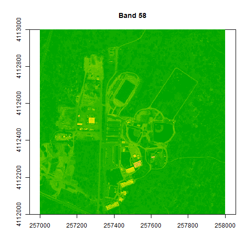
# scale the data as specified in the reflInfo$Scale Factor
rgbStack <- rgbStack/as.integer(reflInfo$Scale_Factor)
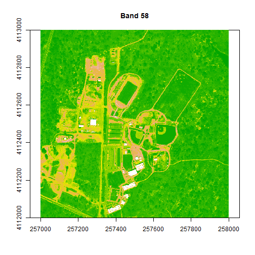
# plot one raster in the stack to make sure things look OK.
plot(rgbStack$Band_58, main="Band 58")
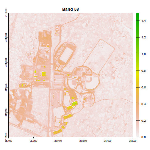
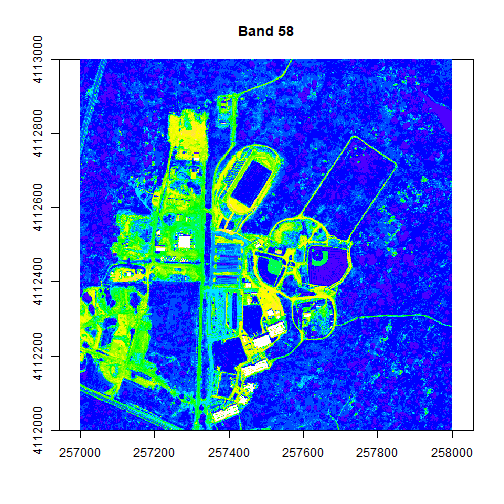
We can play with the color ramps too if we want:
# change the colors of our raster
colors1 <- terrain.colors(25)
image(rgbStack$Band_58, main="Band 58", col=colors1)
# adjust the zlims or the stretch of the image
image(rgbStack$Band_58, main="Band 58", col=colors1, zlim = c(0,.5))
# try a different color palette
colors2 <- topo.colors(15, alpha = 1)
image(rgbStack$Band_58, main="Band 58", col=colors2, zlim=c(0,.5))
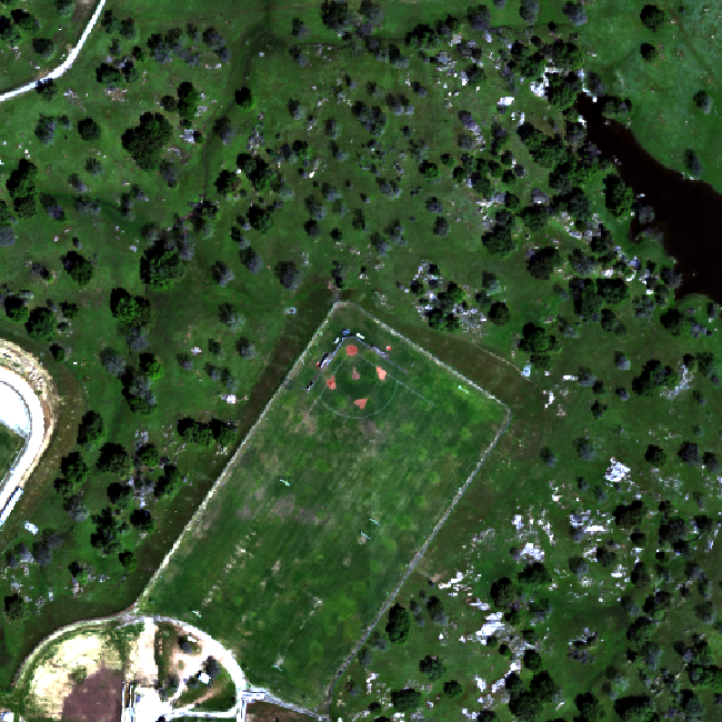
The plotRGB function allows you to combine three bands to create an true-color image.
# create a 3 band RGB image
plotRGB(rgbStack,
        r=1,g=2,b=3,
        stretch = "lin")
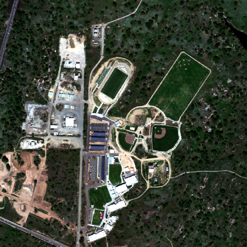
A note about image stretching: Notice that we use the argument stretch="lin" in this plotting function, which automatically stretches the brightness values for us to produce a natural-looking image.
Once you've created your raster, you can export it as a GeoTIFF using writeRaster. You can bring this GeoTIFF into any GIS software, such as QGIS or ArcGIS.
# Write out final raster
# Note: if you set overwrite to TRUE, then you will overwrite (and lose) any older version of the tif file!
writeRaster(rgbStack, file=paste0(data_dir,"NEON_D17_SJER_DP3_257000_4112000_reflectance_2021_RGB.tif"), overwrite=TRUE)
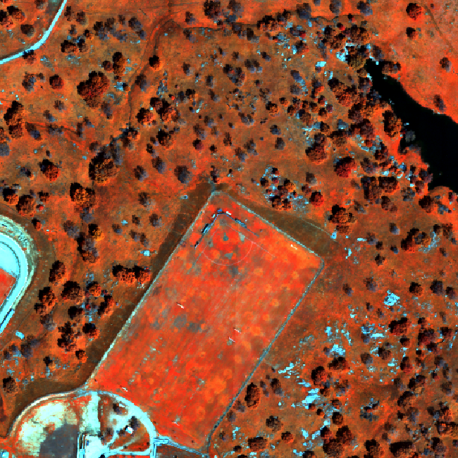
Data Tip - False color and near infrared images: Use the band combinations listed at the top of this page to modify the raster list. What type of image do you get when you change the band values?
Challenge: Other band combinations
Use different band combinations to create other "RGB" images. Suggested band combinations are below for use with the full NEON hyperspectral reflectance datasets (for this example dataset, divide the band number by 4 and round to the nearest whole number):
- Color Infrared/False Color: rgb (90,34,19)
- SWIR, NIR, Red Band: rgb (152,90,58)
- False Color: rgb (363,246,55)
Raster Math - Creating NDVI and other Vegetation Indices in R
In this last part, we will calculate some vegetation indices using raster math in R! We will start by creating NDVI or Normalized Difference Vegetation Index.
About NDVI
NDVI is a ratio between the near infrared (NIR) portion of the electromagnetic spectrum and the red portion of the spectrum.
$$ NDVI = \frac{NIR-RED}{NIR+RED} $$
Please keep in mind that there are different ways to aggregate bands when using hyperspectral data. This example is using individual bands to perform the NDVI calculation. Using individual bands is not necessarily the best way to calculate NDVI from hyperspectral data.
# Calculate NDVI
# select bands to use in calculation (red, NIR)
ndviBands <- c(58,90)
# create raster list and then a stack using those two bands
ndviRast <- lapply(ndviBands,FUN=band2Raster, file = h5_file,
noDataValue=h5NoDataValue,
ext=rastExt, CRS=h5CRS)
ndviStack <- rast(ndviRast)
# make the names pretty
bandNDVINames <- paste("Band_",unlist(ndviBands),sep="")
names(ndviStack) <- bandNDVINames
# view the properties of the new raster stack
ndviStack
## class : SpatRaster
## size : 1000, 1000, 2 (nrow, ncol, nlyr)
## resolution : 1, 1 (x, y)
## extent : 257000, 258000, 4112000, 4113000 (xmin, xmax, ymin, ymax)
## coord. ref. : WGS 84 / UTM zone 11N
## source(s) : memory
## names : Band_58, Band_90
## min values : 0, 11
## max values : 14950, 14887
#calculate NDVI
NDVI <- function(x) {
(x[,2]-x[,1])/(x[,2]+x[,1])
}
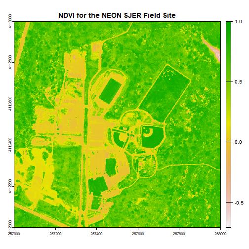
ndviCalc <- app(ndviStack,NDVI)
plot(ndviCalc, main="NDVI for the NEON SJER Field Site")
# Now, play with breaks and colors to create a meaningful map
# add a color map with 4 colors
myCol <- rev(terrain.colors(4)) # use the 'rev()' function to put green as the highest NDVI value
# add breaks to the colormap, including lowest and highest values (4 breaks = 3 segments)
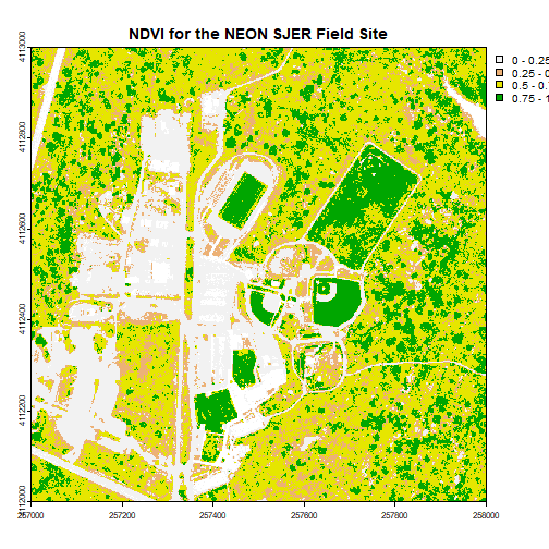
brk <- c(0, .25, .5, .75, 1)
# plot the image using breaks
plot(ndviCalc, main="NDVI for the NEON SJER Field Site", col=myCol, breaks=brk)
Challenge: Work with Indices
Try the following on your own:
- Calculate the Normalized Difference Nitrogen Index (NDNI) using the following equation:
$$ NDNI = \frac{log(\frac{1}{p_{1510}}) - log(\frac{1}{p_{1680}})}{log(\frac{1}{p_{1510}}) + log(\frac{1}{p_{1680}})} $$ 2. Calculate the Enhanced Vegetation Index (EVI). Hint: Look up the formula, and apply the appropriate NEON bands. Hint: You can look at satellite datasets, such as USGS Landsat EVI.
- Explore the bands in the hyperspectral data. What happens if you average reflectance values across multiple Red and NIR bands and then calculate NDVI?