Unsupervised Spectral Classification in Python: KMeans & PCA

In this tutorial, we will use the Spectral Python (SPy) package to run a KMeans unsupervised classification algorithm and then we will run Principal Component Analysis to reduce data dimensionality.

In this tutorial, we will use the Spectral Python (SPy) package to run KMeans unsupervised classification algorithm as well as Principal Component Analysis (PCA).

To learn more about the Spectral Python packages read:

• Spectral Python User Guide.
• Spectral Python Unsupervised Classification.

KMeans Clustering

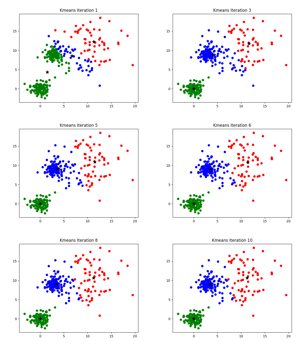
KMeans is an iterative clustering algorithm used to classify unsupervised data (eg. data without a training set) into a specified number of groups. The algorithm begins with an initial set of randomly determined cluster centers. Each pixel in the image is then assigned to the nearest cluster center (using distance in N-space as the distance metric) and each cluster center is then re-computed as the centroid of all pixels assigned to the cluster. This process repeats until a desired stopping criterion is reached (e.g. max number of iterations).

Read more on KMeans clustering from Spectral Python.

To visualize how the algorithm works, it's easier look at a 2D data set. In the example below, watch how the cluster centers shift with progressive iterations,

Principal Component Analysis (PCA) - Dimensionality Reduction

Many of the bands within hyperspectral images are often strongly correlated. The principal components transformation represents a linear transformation of the original image bands to a set of new, uncorrelated features. These new features correspond to the eigenvectors of the image covariance matrix, where the associated eigenvalue represents the variance in the direction of the eigenvector. A very large percentage of the image variance can be captured in a relatively small number of principal components (compared to the original number of bands).

Read more about PCA with Spectral Python.

Let's get started! First, import the required packages.

First, import the required packages and set display preferences:

import h5py
import matplotlib
import neonutilities as nu
import numpy as np
import os
import requests
from spectral import *
from time import time
import dotenv

# Set the data download path, change this path if desired
data_dir = os.path.join(r'C:\data')

For this example, we will download a bidirectional surface reflectance data cube at the SERC site, collected in 2022.

As of June 2026, NEON requires an API token for data downloads, to reduce bot scraping and improve user support. Tokens can be generated in NEON data portal user accounts - log in to your account or create one, and go to the API Tokens section. For best practices in storing and using tokens, follow the instructions here. Once you've set up your token as an environment variable, you can load it using the python-dotenv package as follows, optionally specifying the path to the .env file in load_dotenv().

dotenv.load_dotenv()
token = os.environ.get("NEON_TOKEN")

nu.by_tile_aop(dpid='DP3.30006.002',
               site='SERC',
               year='2022',
               easting=368005,
               northing=4306005,
               include_provisional=True,
               token=token,
               savepath=os.path.join(data_dir)) # save to the home directory under a 'data' subfolder

Provisional NEON data are included. To exclude provisional data, use input parameter include_provisional=False.


Continuing will download 2 NEON data files totaling approximately 659.9 MB. Do you want to proceed? (y/n)  y


Downloading 2 NEON data files totaling approximately 659.9 MB

  0%|                                                                                                                                 | 0/2 [00:00<?, ?it/s]C:\Users\bhass\AppData\Roaming\Python\Python313\site-packages\neonutilities\helper_mods\api_helpers.py:790: UserWarning: Filepaths on Windows are limited to 260 characters. Attempting to download a filepath that is 940 characters long. Set the working or savepath directory to be closer to the root directory or enable long path support in Windows.
  warnings.warn(
C:\Users\bhass\AppData\Roaming\Python\Python313\site-packages\neonutilities\helper_mods\api_helpers.py:790: UserWarning: Filepaths on Windows are limited to 260 characters. Attempting to download a filepath that is 935 characters long. Set the working or savepath directory to be closer to the root directory or enable long path support in Windows.
  warnings.warn(
100%|████████████████████████████████████████████████████████████████████████████████████████████████████████████████████████| 2/2 [00:00<00:00, 117.22it/s]

Let's see what data were downloaded.

# iterate over directory recursively to show path of downloaded h5 file
for root, dirs, files in os.walk(data_dir):
    for name in files:
        if name.endswith('.h5'):
            h5_tile = os.path.join(root, name)
            print(h5_tile)  # printing file name

C:\data\DP3.30006.002\neon-aop-provisional-products\2022\FullSite\D02\2022_SERC_6\L3\Spectrometer\Reflectance\NEON_D02_SERC_DP3_368000_4306000_bidirectional_reflectance.h5
C:\data\DP3.30006.002\neon-aop-provisional-products\2025\FullSite\D02\2025_SERC_7\L3\Spectrometer\Reflectance\NEON_D02_SERC_DP3_368000_4306000_bidirectional_reflectance.h5

# function to download data stored on the internet in a public url to a local file
def download_url(url,download_dir):
    if not os.path.isdir(download_dir):
        os.makedirs(download_dir)
    filename = url.split('/')[-1]
    r = requests.get(url, allow_redirects=True)
    file_object = open(os.path.join(download_dir,filename),'wb')
    file_object.write(r.content)

module_url = "https://raw.githubusercontent.com/NEONScience/NEON-Data-Skills/main/tutorials/Python/AOP/aop_python_modules/neon_aop_hyperspectral.py"
download_url(module_url,'../python_modules')
# os.listdir('../python_modules') #optionally show the contents of this directory to confirm the file downloaded

sys.path.insert(0, '../python_modules')
# import the neon_aop_hyperspectral module, the semicolon supresses an empty plot from displaying
import neon_aop_hyperspectral as neon_hs;

# read in the reflectance data using the aop_h5refl2array function, this may also take a bit of time
start_time = time()
refl, refl_metadata, wavelengths = neon_hs.aop_h5refl2array(h5_tile,'Reflectance')
print("--- It took %s seconds to read in the data ---" % round((time() - start_time),0))

Reading in  C:\data\DP3.30006.002\neon-aop-provisional-products\2025\FullSite\D02\2025_SERC_7\L3\Spectrometer\Reflectance\NEON_D02_SERC_DP3_368000_4306000_bidirectional_reflectance.h5
--- It took 15.0 seconds to read in the data ---

The next few cells show how you can look at the contents, values, and dimensions of the refl_metadata, wavelengths, and refl variables, respectively.

refl_metadata

{'shape': (1000, 1000, 426),
 'no_data_value': -9999.0,
 'scale_factor': 10000.0,
 'bad_band_window1': array([1340, 1445], dtype=int32),
 'bad_band_window2': array([1790, 1955], dtype=int32),
 'projection': b'+proj=UTM +zone=18 +ellps=WGS84 +datum=WGS84 +units=m +no_defs',
 'EPSG': 32618,
 'res': {'pixelWidth': 1.0, 'pixelHeight': 1.0},
 'extent': (368000.0, 369000.0, 4306000.0, 4307000.0),
 'ext_dict': {'xMin': 368000.0,
  'xMax': 369000.0,
  'yMin': 4306000.0,
  'yMax': 4307000.0},
 'source': 'C:\\data\\DP3.30006.002\\neon-aop-provisional-products\\2025\\FullSite\\D02\\2025_SERC_7\\L3\\Spectrometer\\Reflectance\\NEON_D02_SERC_DP3_368000_4306000_bidirectional_reflectance.h5'}

print('First and last 5 center wavelengths, in nm:')
print(wavelengths[:5])
print(wavelengths[-5:])

First and last 5 center wavelengths, in nm:
[381.858398 386.868896 391.879395 396.889893 401.900391]
[2491.281494 2496.291992 2501.30249  2506.312988 2511.323486]

refl.shape

(1000, 1000, 426)

Next let's define a function to clean and subset the data.

def clean_neon_refl_data(data, metadata, wavelengths, subset_factor=1):
    """Clean h5 reflectance data and metadata
    1. set data ignore value (-9999) to NaN
    2. apply reflectance scale factor (10000)
    3. remove bad bands (water vapor band windows + last 10 bands): 
        Band_Window_1_Nanometers = 1340, 1445
        Band_Window_2_Nanometers = 1790, 1955
    4. if subset_factor, subset by that factor
    """
    
    # use copy so original data and metadata doesn't change
    data_clean = data.copy().astype(float)
    metadata_clean = metadata.copy()
    
    #set data ignore value (-9999) to NaN:
    if metadata['no_data_value'] in data:
        nodata_ind = np.where(data_clean==metadata['no_data_value'])
        data_clean[nodata_ind]=np.nan 
    
    #apply reflectance scale factor (divide by 10000)
    data_clean = data_clean/metadata['scale_factor']
    
    #remove bad bands 
    #1. define indices corresponding to min/max center wavelength for each bad band window:
    bb1_ind0 = np.max(np.where(np.asarray(wavelengths<float(metadata['bad_band_window1'][0]))))
    bb1_ind1 = np.min(np.where(np.asarray(wavelengths>float(metadata['bad_band_window1'][1]))))

    bb2_ind0 = np.max(np.where(np.asarray(wavelengths<float(metadata['bad_band_window2'][0]))))
    bb2_ind1 = np.min(np.where(np.asarray(wavelengths>float(metadata['bad_band_window2'][1]))))
    bb3_ind0 = len(wavelengths)-15
    
    #define valid band ranges from indices:
    vb1 = list(range(10,bb1_ind0)); 
    vb2 = list(range(bb1_ind1,bb2_ind0))
    vb3 = list(range(bb2_ind1,bb3_ind0))
    # combine them to get a list of the valid bands
    vbs = vb1 + vb2 + vb3
    # subset by subset_factor (if subset_factor = 1 this will return the original valid_bands list)
    valid_bands_subset = vbs[::subset_factor]

    # subset the reflectance data by the valid_bands_subset
    data_clean = data_clean[:,:,valid_bands_subset]

    # subset the wavelengths by the same valid_bands_subset
    wavelengths_clean =[wavelengths[i] for i in valid_bands_subset]
    
    return data_clean, wavelengths_clean

Now use this function to clean and subset the data, using a subset factor of 2 to start.

# clean the data - remove the band bands and subset
start_time = time()
refl_clean, wavelengths_clean = clean_neon_refl_data(refl, refl_metadata, wavelengths, subset_factor=2)
print("--- It took %s seconds to clean and subset the reflectance data ---" % round((time() - start_time),0))

--- It took 8.0 seconds to clean and subset the reflectance data ---

# Look at the dimensions of the data after cleaning:
print('Cleaned Data Dimensions:',refl_clean.shape)
print('Cleaned Wavelengths:',len(wavelengths_clean))

Cleaned Data Dimensions: (1000, 1000, 173)
Cleaned Wavelengths: 173

start_time = time()
# run kmeans with 5 clusters and 50 iterations
(m,c) = kmeans(refl_clean, 5, 50) 
print("--- It took %s minutes to run kmeans on the reflectance data ---" % round((time() - start_time)/60,1))

spectral:INFO: k-means iteration 1 - 490247 pixels reassigned.
k-means iteration 1 - 490247 pixels reassigned.
spectral:INFO: k-means iteration 2 - 89955 pixels reassigned.
k-means iteration 2 - 89955 pixels reassigned.
spectral:INFO: k-means iteration 3 - 30478 pixels reassigned.
k-means iteration 3 - 30478 pixels reassigned.
spectral:INFO: k-means iteration 4 - 24830 pixels reassigned.
k-means iteration 4 - 24830 pixels reassigned.
spectral:INFO: k-means iteration 5 - 22757 pixels reassigned.
k-means iteration 5 - 22757 pixels reassigned.
spectral:INFO: k-means iteration 6 - 23624 pixels reassigned.
k-means iteration 6 - 23624 pixels reassigned.
spectral:INFO: k-means iteration 7 - 25620 pixels reassigned.
k-means iteration 7 - 25620 pixels reassigned.
spectral:INFO: k-means iteration 8 - 27850 pixels reassigned.
k-means iteration 8 - 27850 pixels reassigned.
spectral:INFO: k-means iteration 9 - 32993 pixels reassigned.
k-means iteration 9 - 32993 pixels reassigned.
spectral:INFO: k-means iteration 10 - 43142 pixels reassigned.
k-means iteration 10 - 43142 pixels reassigned.
spectral:INFO: k-means iteration 11 - 49025 pixels reassigned.
k-means iteration 11 - 49025 pixels reassigned.
spectral:INFO: k-means iteration 12 - 48883 pixels reassigned.
k-means iteration 12 - 48883 pixels reassigned.
spectral:INFO: k-means iteration 13 - 44926 pixels reassigned.
k-means iteration 13 - 44926 pixels reassigned.
spectral:INFO: k-means iteration 14 - 39465 pixels reassigned.
k-means iteration 14 - 39465 pixels reassigned.
spectral:INFO: k-means iteration 15 - 33889 pixels reassigned.
k-means iteration 15 - 33889 pixels reassigned.
spectral:INFO: k-means iteration 16 - 28935 pixels reassigned.
k-means iteration 16 - 28935 pixels reassigned.
spectral:INFO: k-means iteration 17 - 24496 pixels reassigned.
k-means iteration 17 - 24496 pixels reassigned.
spectral:INFO: k-means iteration 18 - 20838 pixels reassigned.
k-means iteration 18 - 20838 pixels reassigned.
spectral:INFO: k-means iteration 19 - 17702 pixels reassigned.
k-means iteration 19 - 17702 pixels reassigned.
spectral:INFO: k-means iteration 20 - 14771 pixels reassigned.
k-means iteration 20 - 14771 pixels reassigned.
spectral:INFO: k-means iteration 21 - 12259 pixels reassigned.
k-means iteration 21 - 12259 pixels reassigned.
spectral:INFO: k-means iteration 22 - 10129 pixels reassigned.
k-means iteration 22 - 10129 pixels reassigned.
spectral:INFO: k-means iteration 23 - 8446 pixels reassigned.
k-means iteration 23 - 8446 pixels reassigned.
spectral:INFO: k-means iteration 24 - 6892 pixels reassigned.
k-means iteration 24 - 6892 pixels reassigned.
spectral:INFO: k-means iteration 25 - 5754 pixels reassigned.
k-means iteration 25 - 5754 pixels reassigned.
spectral:INFO: k-means iteration 26 - 4726 pixels reassigned.
k-means iteration 26 - 4726 pixels reassigned.
spectral:INFO: k-means iteration 27 - 4046 pixels reassigned.
k-means iteration 27 - 4046 pixels reassigned.
spectral:INFO: k-means iteration 28 - 3425 pixels reassigned.
k-means iteration 28 - 3425 pixels reassigned.
spectral:INFO: k-means iteration 29 - 3045 pixels reassigned.
k-means iteration 29 - 3045 pixels reassigned.
spectral:INFO: k-means iteration 30 - 2681 pixels reassigned.
k-means iteration 30 - 2681 pixels reassigned.
spectral:INFO: k-means iteration 31 - 2336 pixels reassigned.
k-means iteration 31 - 2336 pixels reassigned.
spectral:INFO: k-means iteration 32 - 2446 pixels reassigned.
k-means iteration 32 - 2446 pixels reassigned.
spectral:INFO: k-means iteration 33 - 2572 pixels reassigned.
k-means iteration 33 - 2572 pixels reassigned.
spectral:INFO: k-means iteration 34 - 2790 pixels reassigned.
k-means iteration 34 - 2790 pixels reassigned.
spectral:INFO: k-means iteration 35 - 3218 pixels reassigned.
k-means iteration 35 - 3218 pixels reassigned.
spectral:INFO: k-means iteration 36 - 3594 pixels reassigned.
k-means iteration 36 - 3594 pixels reassigned.
spectral:INFO: k-means iteration 37 - 4278 pixels reassigned.
k-means iteration 37 - 4278 pixels reassigned.
spectral:INFO: k-means iteration 38 - 5336 pixels reassigned.
k-means iteration 38 - 5336 pixels reassigned.
spectral:INFO: k-means iteration 39 - 7232 pixels reassigned.
k-means iteration 39 - 7232 pixels reassigned.
spectral:INFO: k-means iteration 40 - 11120 pixels reassigned.
k-means iteration 40 - 11120 pixels reassigned.
spectral:INFO: k-means iteration 41 - 18893 pixels reassigned.
k-means iteration 41 - 18893 pixels reassigned.
spectral:INFO: k-means iteration 42 - 30213 pixels reassigned.
k-means iteration 42 - 30213 pixels reassigned.
spectral:INFO: k-means iteration 43 - 37760 pixels reassigned.
k-means iteration 43 - 37760 pixels reassigned.
spectral:INFO: k-means iteration 44 - 35916 pixels reassigned.
k-means iteration 44 - 35916 pixels reassigned.
spectral:INFO: k-means iteration 45 - 28996 pixels reassigned.
k-means iteration 45 - 28996 pixels reassigned.
spectral:INFO: k-means iteration 46 - 21972 pixels reassigned.
k-means iteration 46 - 21972 pixels reassigned.
spectral:INFO: k-means iteration 47 - 16906 pixels reassigned.
k-means iteration 47 - 16906 pixels reassigned.
spectral:INFO: k-means iteration 48 - 13454 pixels reassigned.
k-means iteration 48 - 13454 pixels reassigned.
spectral:INFO: k-means iteration 49 - 10685 pixels reassigned.
k-means iteration 49 - 10685 pixels reassigned.
spectral:INFO: k-means iteration 50 - 8758 pixels reassigned.
k-means iteration 50 - 8758 pixels reassigned.
spectral:INFO: kmeans terminated with 5 clusters after 50 iterations.
kmeans terminated with 5 clusters after 50 iterations.


--- It took 2.7 minutes to run kmeans on the reflectance data ---

Note that the algorithm still had on the order of 10000 clusters reassigning, when the 50 iterations were reached. You may extend the # of iterations.

Let's try that now:

start_time = time()
# run kmeans with 5 clusters and 40 iterations
(m, c) = kmeans(refl_clean, 5, 40, start_clusters=c) 
print("--- It took %s minutes to run kmeans on the reflectance data ---" % round((time() - start_time)/60,1))

spectral:INFO: k-means iteration 1 - 791183 pixels reassigned.
k-means iteration 1 - 791183 pixels reassigned.
spectral:INFO: k-means iteration 2 - 6618 pixels reassigned.
k-means iteration 2 - 6618 pixels reassigned.
spectral:INFO: k-means iteration 3 - 5791 pixels reassigned.
k-means iteration 3 - 5791 pixels reassigned.
spectral:INFO: k-means iteration 4 - 5019 pixels reassigned.
k-means iteration 4 - 5019 pixels reassigned.
spectral:INFO: k-means iteration 5 - 4565 pixels reassigned.
k-means iteration 5 - 4565 pixels reassigned.
spectral:INFO: k-means iteration 6 - 4180 pixels reassigned.
k-means iteration 6 - 4180 pixels reassigned.
spectral:INFO: k-means iteration 7 - 3956 pixels reassigned.
k-means iteration 7 - 3956 pixels reassigned.
spectral:INFO: k-means iteration 8 - 3625 pixels reassigned.
k-means iteration 8 - 3625 pixels reassigned.
spectral:INFO: k-means iteration 9 - 3271 pixels reassigned.
k-means iteration 9 - 3271 pixels reassigned.
spectral:INFO: k-means iteration 10 - 2978 pixels reassigned.
k-means iteration 10 - 2978 pixels reassigned.
spectral:INFO: k-means iteration 11 - 2612 pixels reassigned.
k-means iteration 11 - 2612 pixels reassigned.
spectral:INFO: k-means iteration 12 - 2348 pixels reassigned.
k-means iteration 12 - 2348 pixels reassigned.
spectral:INFO: k-means iteration 13 - 2138 pixels reassigned.
k-means iteration 13 - 2138 pixels reassigned.
spectral:INFO: k-means iteration 14 - 1863 pixels reassigned.
k-means iteration 14 - 1863 pixels reassigned.
spectral:INFO: k-means iteration 15 - 1728 pixels reassigned.
k-means iteration 15 - 1728 pixels reassigned.
spectral:INFO: k-means iteration 16 - 1539 pixels reassigned.
k-means iteration 16 - 1539 pixels reassigned.
spectral:INFO: k-means iteration 17 - 1305 pixels reassigned.
k-means iteration 17 - 1305 pixels reassigned.
spectral:INFO: k-means iteration 18 - 1206 pixels reassigned.
k-means iteration 18 - 1206 pixels reassigned.
spectral:INFO: k-means iteration 19 - 1060 pixels reassigned.
k-means iteration 19 - 1060 pixels reassigned.
spectral:INFO: k-means iteration 20 - 982 pixels reassigned.
k-means iteration 20 - 982 pixels reassigned.
spectral:INFO: k-means iteration 21 - 913 pixels reassigned.
k-means iteration 21 - 913 pixels reassigned.
spectral:INFO: k-means iteration 22 - 795 pixels reassigned.
k-means iteration 22 - 795 pixels reassigned.
spectral:INFO: k-means iteration 23 - 732 pixels reassigned.
k-means iteration 23 - 732 pixels reassigned.
spectral:INFO: k-means iteration 24 - 671 pixels reassigned.
k-means iteration 24 - 671 pixels reassigned.
spectral:INFO: k-means iteration 25 - 600 pixels reassigned.
k-means iteration 25 - 600 pixels reassigned.
spectral:INFO: k-means iteration 26 - 533 pixels reassigned.
k-means iteration 26 - 533 pixels reassigned.
spectral:INFO: k-means iteration 27 - 469 pixels reassigned.
k-means iteration 27 - 469 pixels reassigned.
spectral:INFO: k-means iteration 28 - 393 pixels reassigned.
k-means iteration 28 - 393 pixels reassigned.
spectral:INFO: k-means iteration 29 - 333 pixels reassigned.
k-means iteration 29 - 333 pixels reassigned.
spectral:INFO: k-means iteration 30 - 305 pixels reassigned.
k-means iteration 30 - 305 pixels reassigned.
spectral:INFO: k-means iteration 31 - 266 pixels reassigned.
k-means iteration 31 - 266 pixels reassigned.
spectral:INFO: k-means iteration 32 - 215 pixels reassigned.
k-means iteration 32 - 215 pixels reassigned.
spectral:INFO: k-means iteration 33 - 171 pixels reassigned.
k-means iteration 33 - 171 pixels reassigned.
spectral:INFO: k-means iteration 34 - 128 pixels reassigned.
k-means iteration 34 - 128 pixels reassigned.
spectral:INFO: k-means iteration 35 - 117 pixels reassigned.
k-means iteration 35 - 117 pixels reassigned.
spectral:INFO: k-means iteration 36 - 101 pixels reassigned.
k-means iteration 36 - 101 pixels reassigned.
spectral:INFO: k-means iteration 37 - 94 pixels reassigned.
k-means iteration 37 - 94 pixels reassigned.
spectral:INFO: k-means iteration 38 - 97 pixels reassigned.
k-means iteration 38 - 97 pixels reassigned.
spectral:INFO: k-means iteration 39 - 77 pixels reassigned.
k-means iteration 39 - 77 pixels reassigned.
spectral:INFO: k-means iteration 40 - 82 pixels reassigned.
k-means iteration 40 - 82 pixels reassigned.
spectral:INFO: kmeans terminated with 5 clusters after 40 iterations.
kmeans terminated with 5 clusters after 40 iterations.


--- It took 2.2 minutes to run kmeans on the reflectance data ---

Passing the initial clusters in sped up the convergence considerably, the second time around.

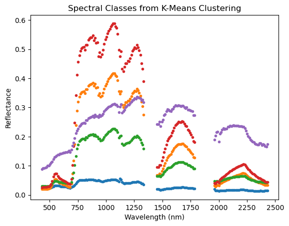
Let's take a look at the new cluster centers c. In this case, these represent spectral signatures of the five clusters (classes) that the data were grouped into. First we can take a look at the shape:

print(c.shape)

(5, 173)

c contains 5 groups of spectral curves with 173 bands (the # of bands we've kept after subsetting and removing the water vapor windows, first 10 noisy bands and last 15 noisy bands). We can plot these spectral classes as follows:

import pylab
pylab.figure()
for i in range(c.shape[0]):
    pylab.plot(wavelengths_clean, c[i],'.')
pylab.show
pylab.title('Spectral Classes from K-Means Clustering')
pylab.xlabel('Wavelength (nm)')
pylab.ylabel('Reflectance');

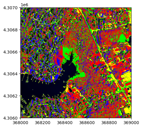
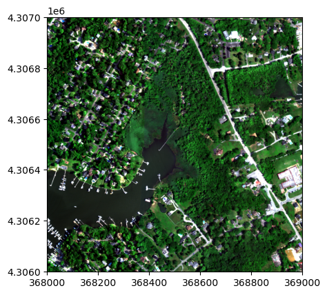
Next, we can look at the classes in map view, as well as a true color image.

view = imshow(refl_clean, bands=(58,34,19),stretch=0.01, classes=m, extent=refl_metadata['extent'])
view.set_display_mode('overlay')
view.class_alpha = 1 #set transparency
view.show_data;

view = imshow(refl_clean, bands=(24,12,4), stretch=0.03, extent=refl_metadata['extent'])
view.show_data;

Challenge Questions: K-Means

1. What do you think the spectral classes in the figure you just created represent?
2. Try using a different number of clusters in the kmeans algorithm (e.g., 3 or 10) to see what spectral classes and classifications result.
3. Try using different (higher) subset_factor in the clean_neon_refl_data function, like 3 or 5. Does this factor change the final classes that are created in the kmeans algorithm? By how much can you subset the data by and still achieve similar classification results?

Principal Component Analysis (PCA)

This next section follows the Spectral Python Dimensionality Reduction section closely.

Many of the bands within hyperspectral images are often strongly correlated. The principal components transformation represents a linear transformation of the original image bands to a set of new, uncorrelated features. These new features correspond to the eigenvectors of the image covariance matrix, where the associated eigenvalue represents the variance in the direction of the eigenvector. A very large percentage of the image variance can be captured in a relatively small number of principal components (compared to the original number of bands) .

pc = principal_components(refl_clean)
pc_view = imshow(pc.cov, extent=refl_metadata['extent'])
xdata = pc.transform(refl_clean)

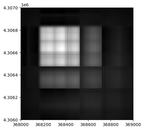
In the covariance matrix display, lighter values indicate strong positive covariance, darker values indicate strong negative covariance, and grey values indicate covariance near zero.

To reduce dimensionality using principal components, we can sort the eigenvalues in descending order and then retain enough eigenvalues (and corresponding eigenvectors) to capture a desired fraction of the total image variance. We then reduce the dimensionality of the image pixels by projecting them onto the remaining eigenvectors. We will choose to retain a minimum of 99.9% of the total image variance.

pc_999 = pc.reduce(fraction=0.999)

# How many eigenvalues are left?
print('# of eigenvalues:',len(pc_999.eigenvalues))

img_pc = pc_999.transform(refl_clean)
print(img_pc.shape)

v = imshow(img_pc[:,:,:3], stretch_all=True, extent=refl_metadata['extent']);

# of eigenvalues: 10
(1000, 1000, 10)

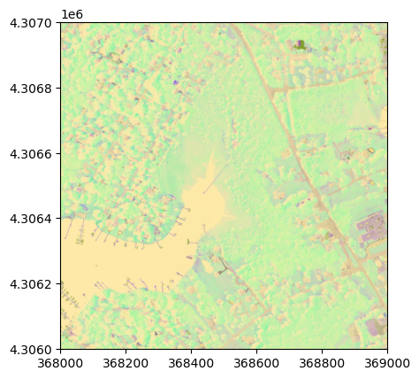
You can see that even though we've only retained a subset of the bands, a lot of the details about the scene are still visible.

If you had training data, you could use a Gaussian maximum likelihood classifier (GMLC) for the reduced principal components to train and classify against the training data.

Challenge Question: PCA

Run the k-means classification after running PCA and see if you get similar results. Does reducing the data dimensionality affect the classification results?