Workshop
Work With Lidar-derived Rasters in R
NEON
This workshop will provide hands on experience with working lidar data in raster format in R. It will cover the basics of what lidar data are and commonly derived data products.
Objectives
After completing this workshop, you will be able to:
- Explain what lidar data are and how they're used in science.
- Describe the key lidar data products - digital surface model, digital terrain model and canopy height model.
- Work with, analyze and export results of lidar derived rasters in R.
Things to Do Before the Workshop
To participant in this workshop, you will need a laptop with the most current version of R and, preferably, RStudio loaded on your computer. For details on setting up R & RStudio in Mac, PC, or Linux operating systems please see Additional Set up Resources below.
Install R Packages
You can chose to install each library individually if you already have some installed. Or you can download the script below and run it to install all libraries at once.
-
raster:
install.packages("raster") -
rgdal:
install.packages("rgdal") -
maptools:
install.packages("maptools") -
ggplot2:
install.packages("ggplot2") -
rgeos:
install.packages("rgeos") -
dplyr:
install.packages("dplyr")
Download The Data
[[nid:6332]] [[nid:6420]]
Background Materials
Workshop Instructors
- Natalie Robinson
- Leah A. Wasser
Schedule
| Time | Topic |
|---|---|
| 12:00 | Working with Raster Data in R |
| 12:45 | Working With Image Formatted Rasters in R |
| 1:15 | The Basics of LiDAR - Light Detection and Ranging - Remote Sensing |
| 1:20 | Explore with Lidar Point Clouds in a free online viewer: plas.io |
| 1:45 | Create a Canopy Height Model from LiDAR-derived Rasters in R |
| 2:30 | Capstone - Create NDVI from GeoTIFFs in R |
| 2:50 | Wrap-up, Feedback, Questions |
Optional resources
QGIS
QGIS is a cross-platform Open Source Geographic Information system.
Online LiDAR Data Viewer (las viewer)
Plas.io is an open source LiDAR data viewer developed by Martin Isenberg of Las Tools and several of his colleagues.
Additional Set Up Instructions
Additional Set Up Instructions
R & RStudio
Prior to the workshop you should have R and, preferably, RStudio installed on your computer.
[[nid:6408]] [[nid:6512]]
Install HDFView
The free HDFView application allows you to explore the contents of an HDF5 file.
To install HDFView:
-
Click to go to the download page.
-
From the section titled HDF-Java 2.1x Pre-Built Binary Distributions select the HDFView download option that matches the operating system and computer setup (32 bit vs 64 bit) that you have. The download will start automatically.
-
Open the downloaded file.
- Mac - You may want to add the HDFView application to your Applications directory.
- Windows - Unzip the file, open the folder, run the .exe file, and follow directions to complete installation.
- Open HDFView to ensure that the program installed correctly.
QGIS (Optional)
QGIS is a cross-platform Open Source Geographic Information system.
Online LiDAR Data/las Viewer (Optional)
Plas.io is a open source LiDAR data viewer developed by Martin Isenberg of Las Tools and several of his colleagues.
| Time | Topic |
|---|---|
| 12:00 | Working with Raster Data in R |
| 12:45 | Working With Image Formatted Rasters in R |
| 1:15 | The Basics of LiDAR - Light Detection and Ranging - Remote Sensing |
| 1:20 | Explore with Lidar Point Clouds in a free online viewer: plas.io |
| 1:45 | Create a Canopy Height Model from LiDAR-derived Rasters in R |
| 2:30 | Capstone - Create NDVI from GeoTIFFs in R |
| 2:50 | Wrap-up, Feedback, Questions |
What is a CHM, DSM and DTM? About Gridded, Raster LiDAR Data
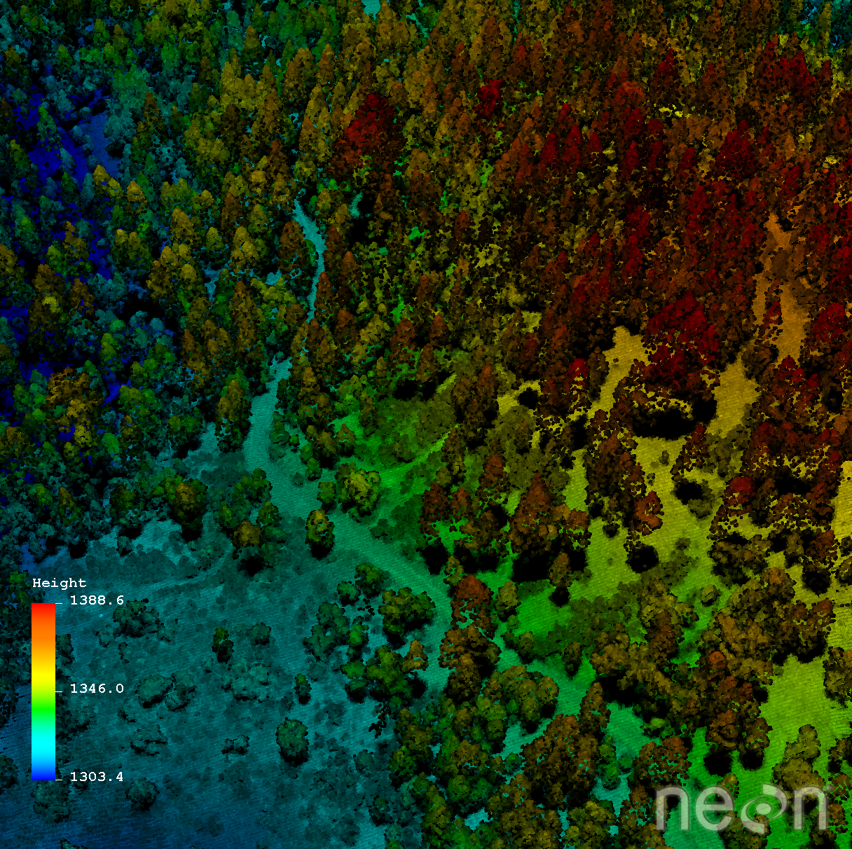
LiDAR Point Clouds
Each point in a LiDAR dataset has a X, Y, Z value and other attributes. The points may be located anywhere in space are not aligned within any particular grid.
LiDAR point clouds are typically available in a .las file format. The .las file format is a compressed format that can better handle the millions of points that are often associated with LiDAR data point clouds.
Common LiDAR Data Products
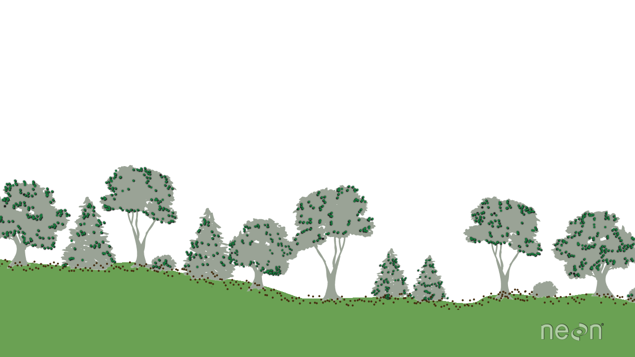
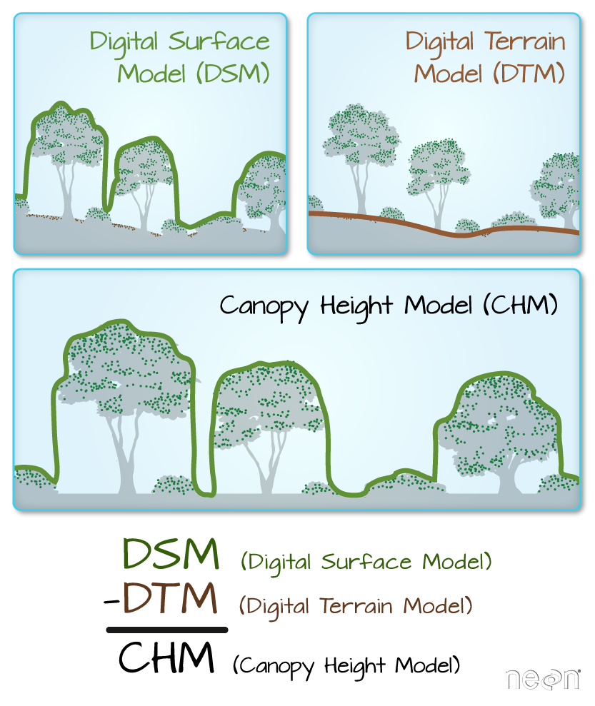
The Digital Terrain Model (DTM) product represents the elevation of the ground, while the Digital Surface Model (DSM) product represents the elevation of the tallest surfaces at that point. Imagine draping a sheet over the canopy of a forest, the Digital Elevation Model (DEM) contours with the heights of the trees where there are trees but the elevation of the ground when there is a clearing in the forest.
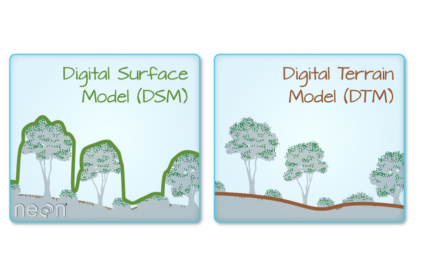
The Canopy height model represents the difference between a Digital Terrain Model and a Digital Surface Model (DSM - DTM = CHM) and gives you the height of the objects (in a forest, the trees) that are on the surface of the earth.
Free Point Cloud Viewers for LiDAR Point Clouds
For more on viewing LiDAR point cloud data using the Plas.io online viewer, see our tutorial Plas.io: Free Online Data Viz to Explore LiDAR Data.
Check out our Structural Diversity tutorial for another useful LiDAR point cloud viewer available through RStudio, Calculating Forest Structural Diversity Metrics from NEON LiDAR Data
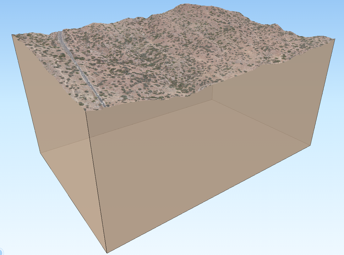
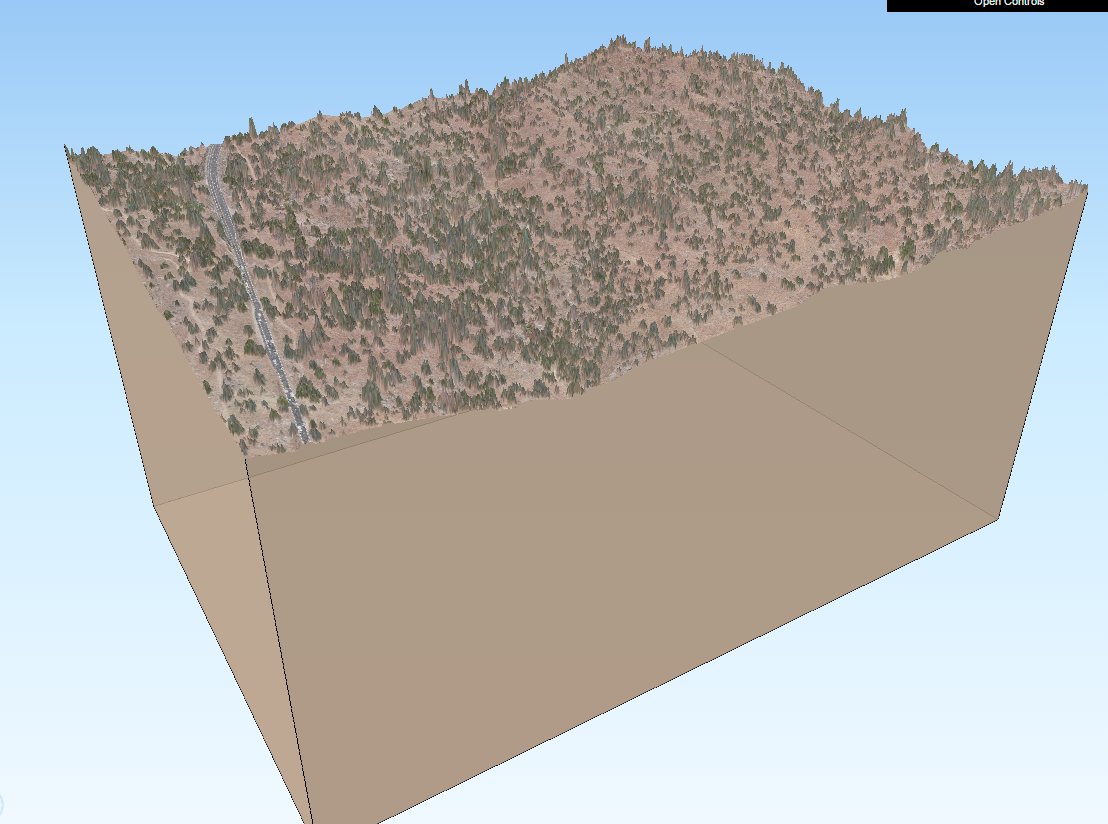
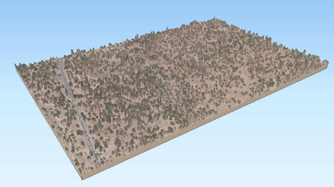
3D Models of NEON Site: SJER (San Joaquin Experimental Range)
Click on the images to view interactive 3D models of San Joaquin Experimental Range site.
 |
 |
 |
Gridded, or Raster, LiDAR Data Products
LiDAR data products are most often worked within a gridded or raster data format. A raster file is a regular grid of cells, all of which are the same size.
A few notes about rasters:
- Each cell is called a pixel.
- And each pixel represents an area on the ground.
- The resolution of the raster represents the area that each pixel represents on the ground. So, for instance if the raster is 1 m resolution, that simple means that each pixel represents a 1m by 1m area on the ground.
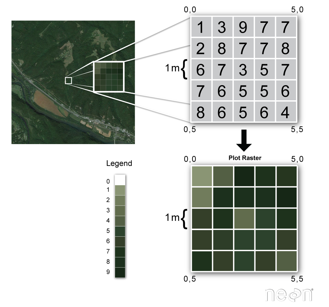
Raster data can have attributes associated with them as well. For instance in a LiDAR-derived digital elevation model (DEM), each cell might represent a particular elevation value. In a LIDAR-derived intensity image, each cell represents a LIDAR intensity value.
LiDAR Related Metadata
In short, when you go to download LiDAR data the first question you should ask is what format the data are in. Are you downloading point clouds that you might have to process? Or rasters that are already processed for you. How do you know?
- Check out the metadata!
- Look at the file format - if you are downloading a .las file, then you are getting points. If it is .tif, then it is a post-processing raster file.
Create Useful Data Products from LiDAR Data
Classify LiDAR Point Clouds
LiDAR data points are vector data. LiDAR point clouds are useful because they tell us something about the heights of objects on the ground. However, how do we know whether a point reflected off of a tree, a bird, a building or the ground? In order to develop products like elevation models and canopy height models, we need to classify individual LiDAR points. We might classify LiDAR points into classes including:
- Ground
- Vegetation
- Buildings
LiDAR point cloud classification is often already done when you download LiDAR point clouds but just know that it’s not to be taken for granted! Programs such as lastools, fusion and terrascan are often used to perform this classification. Once the points are classified, they can be used to derive various LiDAR data products.
Create A Raster From LiDAR Point Clouds
There are different ways to create a raster from LiDAR point clouds.
Point to Raster Methods - Basic Gridding
Let's look one of the most basic ways to create a raster file points - basic gridding. When you perform a gridding algorithm, you are simply calculating a value, using point data, for each pixels in your raster dataset.
- To begin, a grid is placed on top of the LiDAR data in space. Each cell in the grid has the same spatial dimensions. These dimensions represent that particular area on the ground. If we want to derive a 1 m resolution raster from the LiDAR data, we overlay a 1m by 1m grid over the LiDAR data points.
- Within each 1m x 1m cell, we calculate a value to be applied to that cell, using the LiDAR points found within that cell. The simplest method of doing this is to take the max, min or mean height value of all lidar points found within the 1m cell. If we use this approach, we might have cells in the raster that don't contains any lidar points. These cells will have a "no data" value if we process our raster in this way.
Point to Raster Methods - Interpolation
A different approach is to interpolate the value for each cell.
- In this approach we still start with placing the grid on top of the LiDAR data in space.
- Interpolation considers the values of points outside of the cell in addition to points within the cell to calculate a value. Interpolation is useful because it can provide us with some ability to predict or calculate cell values in areas where there are no data (or no points). And to quantify the error associated with those predictions which is useful to know, if you are doing research.
For learning more on how to work with LiDAR and Raster data more generally in R, please refer to the Data Carpentry's Introduction to Geospatial Raster and Vector Data with R lessons.
Image Raster Data in R - An Intro
This tutorial will walk you through the fundamental principles of working with image raster data in R.
Learning Objectives
After completing this activity, you will be able to:
- Import multiple image rasters and create a stack of rasters.
- Plot three band RGB images in R.
- Export single band and multiple band image rasters in R.
Things You’ll Need To Complete This Tutorial
You will need the most current version of R and, preferably, RStudio loaded
on your computer to complete this tutorial.
Install R Packages
-
raster:
install.packages("raster") -
rgdal:
install.packages("rgdal") -
sp:
install.packages("sp")
More on Packages in R – Adapted from Software Carpentry.
Download Data
NEON Teaching Data Subset: Field Site Spatial Data
These remote sensing data files provide information on the vegetation at the National Ecological Observatory Network's San Joaquin Experimental Range and Soaproot Saddle field sites. The entire dataset can be accessed by request from the NEON Data Portal.
Download DatasetThis data download contains several files. You will only need the RGB .tif files for this tutorial. The path to this file is: NEON-DS-Field-Site-Spatial-Data/SJER/RGB/* . The other data files in the downloaded data directory are used for related tutorials. You should set your working directory to the parent directory of the downloaded data to follow the code exactly.
Recommended Reading
You may benefit from reviewing these related resources prior to this tutorial:
Raster Data
Raster or "gridded" data are data that are saved in pixels. In the spatial world, each pixel represents an area on the Earth's surface. An color image raster is a bit different from other rasters in that it has multiple bands. Each band represents reflectance values for a particular color or spectra of light. If the image is RGB, then the bands are in the red, green and blue portions of the electromagnetic spectrum. These colors together create what we know as a full color image.
Work with Multiple Rasters
In
a previous tutorial,
we loaded a single raster into R. We made sure we knew the CRS
(coordinate reference system) and extent of the dataset among other key metadata
attributes. This raster was a Digital Elevation Model so there was only a single
raster that represented the ground elevation in each pixel. When we work with
color images, there are multiple rasters to represent each band. Here we'll learn
to work with multiple rasters together.
Raster Stacks
A raster stack is a collection of raster layers. Each raster layer in the raster stack needs to have the same
- projection (CRS),
- spatial extent and
- resolution.
You might use raster stacks for different reasons. For instance, you might want to group a time series of rasters representing precipitation or temperature into one R object. Or, you might want to create a color images from red, green and blue band derived rasters.
In this tutorial, we will stack three bands from a multi-band image together to create a composite RGB image.
First let's load the R packages that we need: sp and raster.
# load the raster, sp, and rgdal packages
library(raster)
library(sp)
library(rgdal)

# set the working directory to the data
#setwd("pathToDirHere")
wd <- ("~/Git/data/")
setwd(wd)
Next, let's create a raster stack with bands representing
- blue: band 19, 473.8nm
- green: band 34, 548.9nm
- red; band 58, 669.1nm
This can be done by individually assigning each file path as an object.
# import tiffs
band19 <- paste0(wd, "NEON-DS-Field-Site-Spatial-Data/SJER/RGB/band19.tif")
band34 <- paste0(wd, "NEON-DS-Field-Site-Spatial-Data/SJER/RGB/band34.tif")
band58 <- paste0(wd, "NEON-DS-Field-Site-Spatial-Data/SJER/RGB/band58.tif")

# View their attributes to check that they loaded correctly:
band19

## [1] "~/Git/data/NEON-DS-Field-Site-Spatial-Data/SJER/RGB/band19.tif"

band34

## [1] "~/Git/data/NEON-DS-Field-Site-Spatial-Data/SJER/RGB/band34.tif"

band58

## [1] "~/Git/data/NEON-DS-Field-Site-Spatial-Data/SJER/RGB/band58.tif"
Note that if we wanted to create a stack from all the files in a directory (folder)
you can easily do this with the list.files() function. We would use
full.names=TRUE to ensure that R will store the directory path in our list of
rasters.
# create list of files to make raster stack
rasterlist1 <- list.files(paste0(wd,"NEON-DS-Field-Site-Spatial-Data/SJER/RGB", full.names=TRUE))

rasterlist1

## character(0)
Or, if your directory consists of some .tif files and other file types you don't want in your stack, you can ask R to only list those files with a .tif extension.
rasterlist2 <-  list.files(paste0(wd,"NEON-DS-Field-Site-Spatial-Data/SJER/RGB", full.names=TRUE, pattern="tif"))

rasterlist2

## character(0)
Back to creating our raster stack with three bands. We only want three of the
bands in the RGB directory and not the fourth band90, so will create the stack
from the bands we loaded individually. We do this with the stack() function.
# create raster stack
rgbRaster <- stack(band19,band34,band58)

# example syntax for stack from a list
#rstack1 <- stack(rasterlist1)
This has now created a stack that is three rasters thick. Let's view them.
# check attributes
rgbRaster
## class : RasterStack
## dimensions : 502, 477, 239454, 3 (nrow, ncol, ncell, nlayers)
## resolution : 1, 1 (x, y)
## extent : 256521, 256998, 4112069, 4112571 (xmin, xmax, ymin, ymax)
## crs : +proj=utm +zone=11 +datum=WGS84 +units=m +no_defs
## names : band19, band34, band58
## min values : 84, 116, 123
## max values : 13805, 15677, 14343
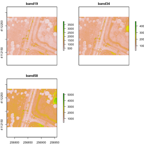
# plot stack
plot(rgbRaster)
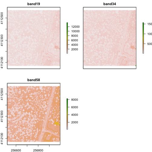
From the attributes we see the CRS, resolution, and extent of all three rasters. The we can see each raster plotted. Notice the different shading between the different bands. This is because the landscape relects in the red, green, and blue spectra differently.
Check out the scale bars. What do they represent?
This reflectance data are radiances corrected for atmospheric effects. The data are typically unitless and ranges from 0-1. NEON Airborne Observation Platform data, where these rasters come from, has a scale factor of 10,000.
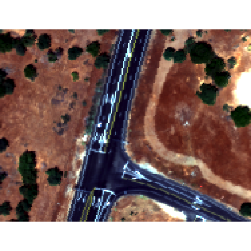
Plot an RGB Image
You can plot a composite RGB image from a raster stack. You need to specify the order of the bands when you do this. In our raster stack, band 19, which is the blue band, is first in the stack, whereas band 58, which is the red band, is last. Thus the order for a RGB image is 3,2,1 to ensure the red band is rendered first as red.
Thinking ahead to next time: If you know you want to create composite RGB images, think about the order of your rasters when you make the stack so the RGB=1,2,3.
We will plot the raster with the rgbRaster() function and the need these
following arguments:
- R object to plot
- which layer of the stack is which color
- stretch: allows for increased contrast. Options are "lin" & "hist".
Let's try it.
# plot an RGB version of the stack
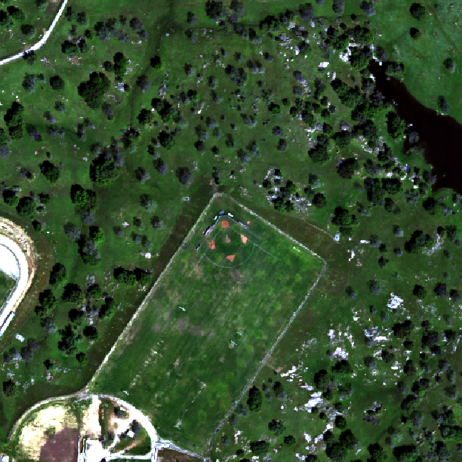
plotRGB(rgbRaster,r=3,g=2,b=1, stretch = "lin")
Note: read the raster package documentation for other arguments that can be
added (like scale) to improve or modify the image.
Explore Raster Values - Histograms
You can also explore the data. Histograms allow us to view the distrubiton of values in the pixels.
# view histogram of reflectance values for all rasters
hist(rgbRaster)

## Warning in .hist1(raster(x, y[i]), maxpixels = maxpixels, main =
## main[y[i]], : 42% of the raster cells were used. 100000 values used.

## Warning in .hist1(raster(x, y[i]), maxpixels = maxpixels, main =
## main[y[i]], : 42% of the raster cells were used. 100000 values used.

## Warning in .hist1(raster(x, y[i]), maxpixels = maxpixels, main =
## main[y[i]], : 42% of the raster cells were used. 100000 values used.
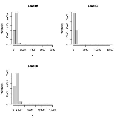
Note about the warning messages: R defaults to only showing the first 100,000 values in the histogram so if you have a large raster you may not be seeing all the values. This saves your from long waits, or crashing R, if you have large datasets.
Crop Rasters
You can crop all rasters within a raster stack the same way you'd do it with a single raster.
# determine the desired extent
rgbCrop <- c(256770.7,256959,4112140,4112284)

# crop to desired extent
rgbRaster_crop <- crop(rgbRaster, rgbCrop)

# view cropped stack
plot(rgbRaster_crop)
Raster Bricks in R
In our rgbRaster object we have a list of rasters in a stack. These rasters
are all the same extent, CRS and resolution. By creating a raster brick we
will create one raster object that contains all of the rasters so that we can
use this object to quickly create RGB images. Raster bricks are more efficient
objects to use when processing larger datasets. This is because the computer
doesn't have to spend energy finding the data - it is contained within the object.
# create raster brick
rgbBrick <- brick(rgbRaster)

# check attributes
rgbBrick

## class      : RasterBrick
## dimensions : 502, 477, 239454, 3  (nrow, ncol, ncell, nlayers)
## resolution : 1, 1  (x, y)
## extent     : 256521, 256998, 4112069, 4112571  (xmin, xmax, ymin, ymax)
## crs        : +proj=utm +zone=11 +datum=WGS84 +units=m +no_defs
## source     : memory
## names      : band19, band34, band58
## min values :     84,    116,    123
## max values :  13805,  15677,  14343
While the brick might seem similar to the stack (see attributes above), we can see that it's very different when we look at the size of the object.
- the brick contains all of the data stored in one object
- the stack contains links or references to the files stored on your computer
Use object.size() to see the size of an R object.
# view object size
object.size(rgbBrick)
## 5762000 bytes
object.size(rgbRaster)
## 49984 bytes
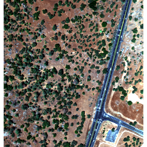
# view raster brick
plotRGB(rgbBrick,r=3,g=2,b=1, stretch = "Lin")

Notice the faster plotting? For a smaller raster like this the difference is slight, but for larger raster it can be considerable.
Write to GeoTIFF
We can write out the raster in GeoTIFF format as well. When we do this it will copy the CRS, extent and resolution information so the data will read properly into a GIS program as well. Note that this writes the raster in the order they are in. In our case, the blue (band 19) is first but most programs expect the red band first (RGB).
One way around this is to generate a new raster stack with the rasters in the proper order - red, green and blue format. Or, just always create your stacks R->G->B to start!!!
# Make a new stack in the order we want the data in
orderRGBstack <- stack(rgbRaster$band58,rgbRaster$band34,rgbRaster$band19)

# write the geotiff
# change overwrite=TRUE to FALSE if you want to make sure you don't overwrite your files!
writeRaster(orderRGBstack,paste0(wd,"NEON-DS-Field-Site-Spatial-Data/SJER/RGB/rgbRaster.tif"),"GTiff", overwrite=TRUE)
Import A Multi-Band Image into R
You can import a multi-band image into R too. To do this, you import the file as a stack rather than a raster (which brings in just one band). Let's import the raster than we just created above.
# import multi-band raster as stack
multiRasterS <- stack(paste0(wd,"NEON-DS-Field-Site-Spatial-Data/SJER/RGB/rgbRaster.tif"))

# import multi-band raster direct to brick
multiRasterB <- brick(paste0(wd,"NEON-DS-Field-Site-Spatial-Data/SJER/RGB/rgbRaster.tif"))

# view raster
plot(multiRasterB)
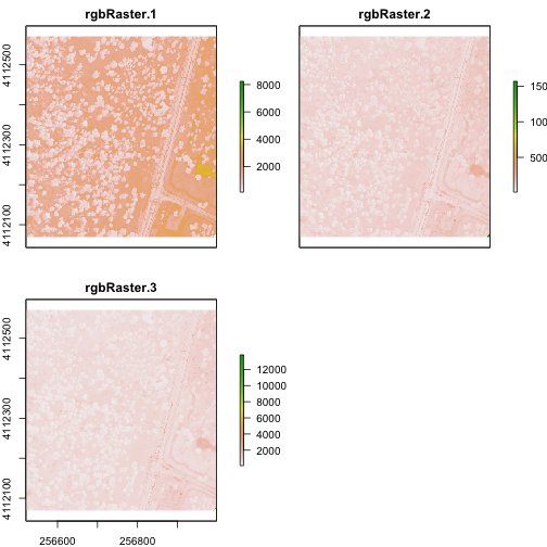
plotRGB(multiRasterB,r=1,g=2,b=3, stretch="lin")

The Basics of LiDAR - Light Detection and Ranging - Remote Sensing
LiDAR or Light Detection and Ranging is an active remote sensing system that can be used to measure vegetation height across wide areas. This page will introduce fundamental LiDAR (or lidar) concepts including:
- What LiDAR data are.
- The key attributes of LiDAR data.
- How LiDAR data are used to measure trees.
The Story of LiDAR
Key Concepts
Why LiDAR
Scientists often need to characterize vegetation over large regions to answer research questions at the ecosystem or regional scale. Therefore, we need tools that can estimate key characteristics over large areas because we don’t have the resources to measure each and every tree or shrub.
Remote sensing means that we aren’t actually physically measuring things with our hands. We are using sensors which capture information about a landscape and record things that we can use to estimate conditions and characteristics. To measure vegetation or other data across large areas, we need remote sensing methods that can take many measurements quickly, using automated sensors.
LiDAR, or Light Detection And Ranging (sometimes also referred to as active laser scanning) is one remote sensing method that can be used to map structure including vegetation height, density and other characteristics across a region. LiDAR directly measures the height and density of vegetation on the ground making it an ideal tool for scientists studying vegetation over large areas.
How LiDAR Works
How Does LiDAR Work?
LiDAR is an active remote sensing system. An active system means that the system itself generates energy - in this case, light - to measure things on the ground. In a LiDAR system, light is emitted from a rapidly firing laser. You can imagine light quickly strobing (or pulsing) from a laser light source. This light travels to the ground and reflects off of things like buildings and tree branches. The reflected light energy then returns to the LiDAR sensor where it is recorded.
A LiDAR system measures the time it takes for emitted light to travel to the ground and back, called the two-way travel time. That time is used to calculate distance traveled. Distance traveled is then converted to elevation. These measurements are made using the key components of a lidar system including a GPS that identifies the X,Y,Z location of the light energy and an Inertial Measurement Unit (IMU) that provides the orientation of the plane in the sky (roll, pitch, and yaw).
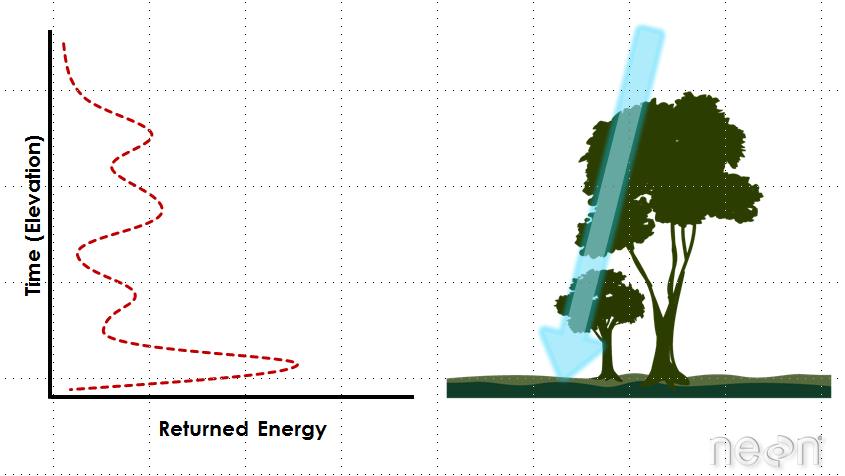
How Light Energy Is Used to Measure Trees
Light energy is a collection of photons. As photon that make up light moves towards the ground, they hit objects such as branches on a tree. Some of the light reflects off of those objects and returns to the sensor. If the object is small, and there are gaps surrounding it that allow light to pass through, some light continues down towards the ground. Because some photons reflect off of things like branches but others continue down towards the ground, multiple reflections (or "returns") may be recorded from one pulse of light.
LiDAR waveforms
The distribution of energy that returns to the sensor creates what we call a waveform. The amount of energy that returned to the LiDAR sensor is known as "intensity". The areas where more photons or more light energy returns to the sensor create peaks in the distribution of energy. Theses peaks in the waveform often represent objects on the ground like - a branch, a group of leaves or a building.
How Scientists Use LiDAR Data
There are many different uses for LiDAR data.
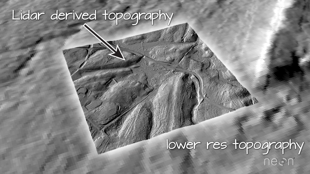
- LiDAR data classically have been used to derive high resolution elevation data models
- LiDAR data have also been used to derive information about vegetation structure including:
- Canopy Height
- Canopy Cover
- Leaf Area Index
- Vertical Forest Structure
- Species identification (if a less dense forests with high point density LiDAR)
Discrete vs. Full Waveform LiDAR
A waveform or distribution of light energy is what returns to the LiDAR sensor. However, this return may be recorded in two different ways.
- A Discrete Return LiDAR System records individual (discrete) points for the peaks in the waveform curve. Discrete return LiDAR systems identify peaks and record a point at each peak location in the waveform curve. These discrete or individual points are called returns. A discrete system may record 1-11+ returns from each laser pulse.
- A Full Waveform LiDAR System records a distribution of returned light energy. Full waveform LiDAR data are thus more complex to process, however they can often capture more information compared to discrete return LiDAR systems. One example research application for full waveform LiDAR data includes mapping or modelling the understory of a canopy.
LiDAR File Formats
Whether it is collected as discrete points or full waveform, most often LiDAR data are available as discrete points. A collection of discrete return LiDAR points is known as a LiDAR point cloud.
The commonly used file format to store LIDAR point cloud data is called ".las" which is a format supported by the American Society of Photogrammetry and Remote Sensing (ASPRS). Recently, the .laz format has been developed by Martin Isenberg of LasTools. The differences is that .laz is a highly compressed version of .las.
Data products derived from LiDAR point cloud data are often raster files that may be in GeoTIFF (.tif) formats.
LiDAR Data Attributes: X, Y, Z, Intensity and Classification
LiDAR data attributes can vary, depending upon how the data were collected and processed. You can determine what attributes are available for each lidar point by looking at the metadata. All lidar data points will have an associated X,Y location and Z (elevation) values. Most lidar data points will have an intensity value, representing the amount of light energy recorded by the sensor.
Some LiDAR data will also be "classified" -- not top secret, but with specifications about what the data represent. Classification of LiDAR point clouds is an additional processing step. Classification simply represents the type of object that the laser return reflected off of. So if the light energy reflected off of a tree, it might be classified as "vegetation" point. And if it reflected off of the ground, it might be classified as "ground" point.
Some LiDAR products will be classified as "ground/non-ground". Some datasets will be further processed to determine which points reflected off of buildings and other infrastructure. Some LiDAR data will be classified according to the vegetation type.
Exploring 3D LiDAR data in a free Online Viewer
Check out our tutorial on viewing LiDAR point cloud data using the Plas.io online viewer: Plas.io: Free Online Data Viz to Explore LiDAR Data. The Plas.io viewer used in this tutorial was developed by Martin Isenberg of Las Tools and his colleagues.
Summary
- A LiDAR system uses a laser, a GPS and an IMU to estimate the heights of objects on the ground.
- Discrete LiDAR data are generated from waveforms -- each point represent peak energy points along the returned energy.
- Discrete LiDAR points contain an x, y and z value. The z value is what is used to generate height.
- LiDAR data can be used to estimate tree height and even canopy cover using various methods.
Additional Resources
- What is the LAS format?
- Using .las with Python? las: python ingest
- Specifications for las v1.3
Create a Canopy Height Model from Lidar-derived rasters in R
A common analysis using lidar data are to derive top of the canopy height values from the lidar data. These values are often used to track changes in forest structure over time, to calculate biomass, and even leaf area index (LAI). Let's dive into the basics of working with raster formatted lidar data in R!
Learning Objectives
After completing this tutorial, you will be able to:
- Work with digital terrain model (DTM) & digital surface model (DSM) raster files.
- Carry out basic raster math using the
terrapackage. - Create a canopy height model (CHM) raster from DTM & DSM rasters.
- Understand the basics of the pit-free CHM algoirthm used to generate NEON's Ecosystem Structure data product.
Things You’ll Need To Complete This Tutorial
You will need the most current version of R and, preferably, RStudio loaded
on your computer to complete this tutorial.
As of June 2026, NEON requires an API token for data downloads, to reduce bot scraping and improve user support. Tokens can be generated in NEON data portal user accounts - log in to your account or create one, and go to the API Tokens section. For best practices in storing and using tokens, follow the instructions here.
Install R Packages
-
terra:
install.packages("terra") -
neonUtilities:
install.packages("neonUtilities")
More on Packages in R - Adapted from Software Carpentry.
Download Data
Lidar elevation raster data are downloaded using the R neonUtilities::byTileAOP() function in the script.
These remote sensing data files provide information on the vegetation at the National Ecological Observatory Network's San Joaquin Experimental Range site. The entire datasets can be accessed from the NEON Data Portal.
R Script & Challenge Code: NEON data lessons often contain challenges to reinforce skills. If available, the code for challenge solutions is found in the downloadable R script of the entire lesson, available in the footer of each lesson page.
Recommended Reading
What is a CHM, DSM and DTM? About Gridded, Raster LiDAR DataCreate a Lidar-derived Canopy Height Model (CHM)
The National Ecological Observatory Network (NEON) provides lidar-derived data products including the 1) Digital Terrain Model and Digital Surface Model (DTM/DSM), 2) Slope and Aspect, and 3) Ecosystem Structure or Canopy Height Model (CHM). These products come in the GeoTIFF format, which is a .tif raster format that is spatially located on the earth.
In this tutorial, we create a Canopy Height Model. The Canopy Height Model (CHM), represents the heights of the trees on the ground. We can derive the CHM by subtracting the ground elevation from the elevation of the top of the surface (or the tops of the trees).
We will use the terra R package to work with the the lidar-derived Digital
Surface Model (DSM) and the Digital Terrain Model (DTM).
# Load needed packages and set API token

library(terra)

library(neonUtilities)

token <- Sys.getenv("NEON_TOKEN")
Set the data directory where downloaded data will be saved.
data_dir="~/data/" #This will depend on your local environment
We can use the neonUtilities function byTileAOP to download a single DTM and DSM tile at SJER. Both the DTM and DSM are delivered under the Elevation - LiDAR (DP3.30024.001) data product.
You can run help(byTileAOP) to see more details on what the various inputs are. For this exercise, we'll specify the UTM Easting and Northing to be (257500, 4112500), which will download the tile with the lower left corner (257000,4112000). By default, the function will check the size total size of the download and ask you whether you wish to proceed (y/n). You can set check.size=FALSE if you want to download without a prompt. This example will not be very large (~8MB), since it is only downloading two single-band rasters (plus some associated metadata).
byTileAOP(dpID='DP3.30024.001',
          site='SJER',
          year='2021',
          easting=257500,
          northing=4112500,
          check.size=TRUE, # set to FALSE if you don't want to enter y/n
          savepath = data_dir,
          token=token)

## Downloading 2 files

##
|
| | 0%
|
|==============================================================================================| 100%
## Successfully downloaded 2 files to ~/data//DP3.30024.001
This file will be downloaded into a nested subdirectory under the ~/data folder, inside a folder named DP3.30024.001 (the Data Product ID). The files should show up in these locations: ~/data/DP3.30024.001/neon-aop-products/2021/FullSite/D17/2021_SJER_5/L3/DiscreteLidar/DSMGtif/NEON_D17_SJER_DP3_257000_4112000_DSM.tif and ~/data/DP3.30024.001/neon-aop-products/2021/FullSite/D17/2021_SJER_5/L3/DiscreteLidar/DTMGtif/NEON_D17_SJER_DP3_257000_4112000_DTM.tif.
Now we can read in the files. You can move the files to a different location (eg. shorten the path), but make sure to change the path that points to the file accordingly.
# Define the DSM and DTM file names, including the full path

dsm_file <- paste0(data_dir,"DP3.30024.001/neon-aop-products/2021/FullSite/D17/2021_SJER_5/L3/DiscreteLidar/DSMGtif/NEON_D17_SJER_DP3_257000_4112000_DSM.tif")

dtm_file <- paste0(data_dir,"DP3.30024.001/neon-aop-products/2021/FullSite/D17/2021_SJER_5/L3/DiscreteLidar/DTMGtif/NEON_D17_SJER_DP3_257000_4112000_DTM.tif")
First, we will read in the Digital Surface Model (DSM). The DSM represents the elevation of the top of the objects on the ground (trees, buildings, etc).
# assign raster to object

dsm <- rast(dsm_file)


# view info about the raster.

dsm

## class       : SpatRaster
## size        : 1000, 1000, 1  (nrow, ncol, nlyr)
## resolution  : 1, 1  (x, y)
## extent      : 257000, 258000, 4112000, 4113000  (xmin, xmax, ymin, ymax)
## coord. ref. : WGS 84 / UTM zone 11N (EPSG:32611)
## source      : NEON_D17_SJER_DP3_257000_4112000_DSM.tif
## name        : NEON_D17_SJER_DP3_257000_4112000_DSM

# plot the DSM

plot(dsm, main="Lidar Digital Surface Model \n SJER, California")
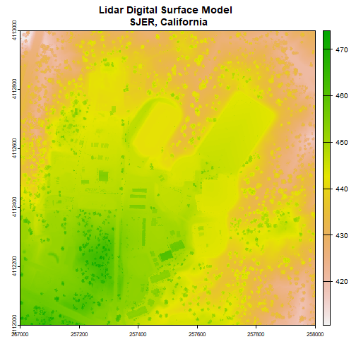
Note the resolution, extent, and coordinate reference system (CRS) of the raster. To do later steps, our DTM will need to be the same.
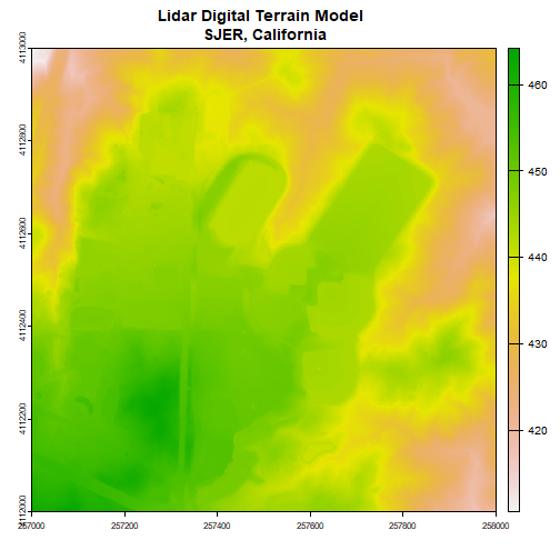
Next, we will import the Digital Terrain Model (DTM) for the same area. The DTM represents the ground (terrain) elevation.
# import the digital terrain model

dtm <- rast(dtm_file)


plot(dtm, main="Lidar Digital Terrain Model \n SJER, California")
With both of these rasters now loaded, we can create the Canopy Height Model (CHM). The CHM represents the difference between the DSM and the DTM or the height of all objects on the surface of the earth.
To do this we perform some basic raster math to calculate the CHM. You can perform the same raster math in a GIS program like QGIS.
When you do the math, make sure to subtract the DTM from the DSM or you'll get trees with negative heights!
# use raster math to create CHM

chm <- dsm - dtm


# view CHM attributes

chm

## class       : SpatRaster
## size        : 1000, 1000, 1  (nrow, ncol, nlyr)
## resolution  : 1, 1  (x, y)
## extent      : 257000, 258000, 4112000, 4113000  (xmin, xmax, ymin, ymax)
## coord. ref. : WGS 84 / UTM zone 11N (EPSG:32611)
## source(s)   : memory
## varname     : NEON_D17_SJER_DP3_257000_4112000_DSM
## name        : NEON_D17_SJER_DP3_257000_4112000_DSM
## min value   :                                    0
## max value   :                            24.130005

plot(chm, main="Lidar CHM - SJER, California")
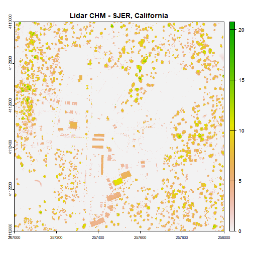
We've now created a CHM from our DSM and DTM. What do you notice about the canopy cover at this location in the San Joaquin Experimental Range?
Pit-Free Canopy Height Model
Note that NEON's Ecosystem Structure (or CHM) data product is not a simple difference between the DSM and DTM. Directly subtracting the DTM from the DSM to determine a CHM can introduce artifacts into the CHM known as data pits. Data pits manifest as abnormally low elevation pixels within a tree crown and underestimate the true canopy height, and are a commonly observed problem in CHMs derived from LiDAR. To address this issue, NEON uses a "pit-free" CHM algorithm, following the method of Khosravipour et al. (2014). To read more about how the NEON CHM is derived, please reference the Ecosystem Structure ATBD.
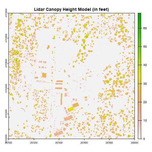
Challenge: Basic Raster Math
Convert the CHM from meters to feet and plot it.
We can write out the CHM as a GeoTiff using the writeRaster() function.
# write out the CHM in tiff format.

writeRaster(chm,paste0(wd,"CHM_SJER.tif"),"GTiff")
We've now successfully created a canopy height model using basic raster math -- in
R! We can bring the CHM_SJER.tif file into QGIS (or any GIS program) and look
at it.
Consider checking out the tutorial Compare tree height measured from the ground to a Lidar-based Canopy Height Model to compare a LiDAR-derived CHM with ground-based observations!
References:
Khosravipour, A., Skidmore, A. K., Isenburg, M., Wang, T., & Hussin, Y. A. (2014). Generating pit-free canopy height models from airborne lidar. Photogrammetric Engineering & Remote Sensing, 80(9), 863–872.