Select pixels and compare spectral signatures in R

In this tutorial, we will learn how to plot spectral signatures of several different land cover types using an interactive click feature of the terra package.

Getting Started

First, we need to load our required packages and set the working directory.

# load required packages

library(rhdf5)

library(reshape2)

library(terra)

library(plyr)

library(ggplot2)

library(grDevices)



# set working directory, you can change this if desired

wd <- "~/data/" 

setwd(wd)

Download the reflectance tile, if you haven't already, using neonUtilities::byTileAOP:

byTileAOP(dpID = 'DP3.30006.001',

          site = 'SJER',

          year = '2021',

          easting = 257500,

          northing = 4112500,

          savepath = wd)

And then we can read in the hyperspectral hdf5 data. We will also collect a few other important pieces of information (band wavelengths and scaling factor) while we're at it.

# define filepath to the hyperspectral dataset

h5_file <- paste0(wd,"DP3.30006.001/neon-aop-products/2021/FullSite/D17/2021_SJER_5/L3/Spectrometer/Reflectance/NEON_D17_SJER_DP3_257000_4112000_reflectance.h5")



# read in the wavelength information from the HDF5 file

wavelengths <- h5read(h5_file,"/SJER/Reflectance/Metadata/Spectral_Data/Wavelength")



# grab scale factor from the Reflectance attributes

reflInfo <- h5readAttributes(h5_file,"/SJER/Reflectance/Reflectance_Data" )



scaleFact <- reflInfo$Scale_Factor

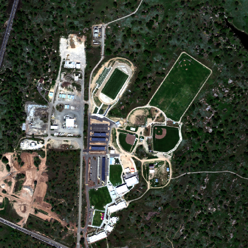
Now, we will read in the RGB image that we created in an earlier tutorial and plot it.

# read in RGB image as a 'stack' rather than a plain 'raster'

rgbStack <- rast(paste0(wd,"NEON_hyperspectral_tutorial_example_RGB_image.tif"))



# plot as RGB image, with a linear stretch

plotRGB(rgbStack,
        r=1,g=2,b=3, scale=300, 
        stretch = "lin")

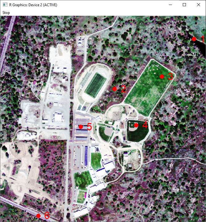
Interactive click Function from the terra Package

Next, we use an interactive clicking function to identify the pixels that we want to extract spectral signatures for. To follow along with this tutorial, we suggest the following six cover types (exact locations shown in the image below).

1. Water
2. Tree canopy (avoid the shaded northwestern side of the tree)
3. Irrigated grass
4. Bare soil (baseball diamond infield)
5. Building roof (blue)
6. Road

As shown here:

For this next part, if you are following along in RStudio, you will need to enter these line below directly in the Console. dev.new(noRStudioGD = TRUE) will open up a separate window for plotting, which is where you will click the pixels to extract spectra, using the terra::click functionality.

dev.new(noRStudioGD = TRUE)

Now we can create our RGB plot, and start clicking on this in the pop-out Graphics window.

# change plotting parameters to better see the points and numbers generated from clicking

par(col="red", cex=2)



# use a histogram stretch in order to provide more contrast for selecting pixels

plotRGB(rgbStack, r=1, g=2, b=3, scale=300, stretch = "hist") 



# use the 'click' function

c <- click(rgbStack, n = 6, id=TRUE, xy=TRUE, cell=TRUE, type="p", pch=16, col="red", col.lab="red")

Once you have clicked your six points, the graphics window should close. If you want to choose new points, or if you accidentally clicked a point that you didn't intend to, run the previous 2 chunks of code again to re-start.

The click() function identifies the cell number that you clicked, but in order to extract spectral signatures, we need to convert that cell number into a row and column, as shown here:

# convert raster cell number into row and column (used to extract spectral signature below)

c$row <- c$cell%/%nrow(rgbStack)+1 # add 1 because R is 1-indexed

c$col <- c$cell%%ncol(rgbStack)

Extract Spectral Signatures from HDF5 file

Next, we will loop through each of the cells that and use the h5read() function to extract the reflectance values of all bands from the given pixel (row and column).

# create a new dataframe from the band wavelengths so that we can add the reflectance values for each cover type

pixel_df <- as.data.frame(wavelengths)

# loop through each of the cells that we selected

for(i in 1:length(c$cell)){
# extract spectral values from a single pixel
aPixel <- h5read(h5_file,"/SJER/Reflectance/Reflectance_Data",
                 index=list(NULL,c$col[i],c$row[i]))

# scale reflectance values from 0-1
aPixel <- aPixel/as.vector(scaleFact)

# reshape the data and turn into dataframe
b <- adply(aPixel,c(1))

# rename the column that we just created
names(b)[2] <- paste0("Point_",i)

# add reflectance values for this pixel to our combined data.frame called pixel_df
pixel_df <- cbind(pixel_df,b[2])
}

Plot Spectral signatures using ggplot2

Finally, we have everything that we need to plot the spectral signatures for each of the pixels that we clicked. In order to color our lines by the different land cover types, we will first reshape our data using the melt() function, then plot the spectral signatures.

# Use the melt() function to reshape the dataframe into a format that ggplot prefers

pixel.melt <- reshape2::melt(pixel_df, id.vars = "wavelengths", value.name = "Reflectance")

# Now, let's plot the spectral signatures!

ggplot()+
  geom_line(data = pixel.melt, mapping = aes(x=wavelengths, y=Reflectance, color=variable), lwd=1.5)+
  scale_colour_manual(values = c("blue3","green4","green2","tan4","grey50","black"),
                      labels = c("Water","Tree","Grass","Soil","Roof","Road"))+
  labs(color = "Cover Type")+
  ggtitle("Land cover spectral signatures")+
  theme(plot.title = element_text(hjust = 0.5, size=20))+
  xlab("Wavelength")

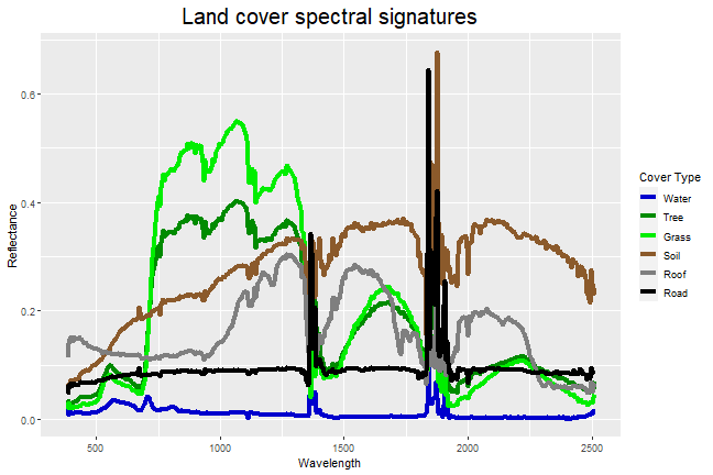
Nice! However, there seems to be something weird going on in the wavelengths near ~1400nm and ~1850 nm...

Atmospheric Absorption Bands

Those irregularities around 1400nm and 1850 nm are two major atmospheric absorption bands - regions where gasses in the atmosphere (primarily carbon dioxide and water vapor) absorb radiation, and therefore, obscure the reflected radiation that the imaging spectrometer measures. Fortunately, the lower and upper bound of each of those atmospheric absorption bands is specified in the HDF5 file. Let's read those bands and plot rectangles where the reflectance measurements are obscured by atmospheric absorption.

# grab reflectance metadata (which contains absorption band limits)

reflMetadata <- h5readAttributes(h5_file,"/SJER/Reflectance" )

ab1 <- reflMetadata$Band_Window_1_Nanometers

ab2 <- reflMetadata$Band_Window_2_Nanometers

# Plot spectral signatures again with grey rectangles highlighting the absorption bands

ggplot()+
  geom_line(data = pixel.melt, mapping = aes(x=wavelengths, y=Reflectance, color=variable), lwd=1.5)+
  geom_rect(mapping=aes(ymin=min(pixel.melt$Reflectance),ymax=max(pixel.melt$Reflectance), xmin=ab1[1], xmax=ab1[2]), color="black", fill="grey40", alpha=0.8)+
  geom_rect(mapping=aes(ymin=min(pixel.melt$Reflectance),ymax=max(pixel.melt$Reflectance), xmin=ab2[1], xmax=ab2[2]), color="black", fill="grey40", alpha=0.8)+
  scale_colour_manual(values = c("blue3","green4","green2","tan4","grey50","black"),
                      labels = c("Water","Tree","Grass","Soil","Roof","Road"))+
  labs(color = "Cover Type")+
  ggtitle("Land cover spectral signatures with\n atmospheric absorption bands greyed out")+
  theme(plot.title = element_text(hjust = 0.5, size=20))+
  xlab("Wavelength")

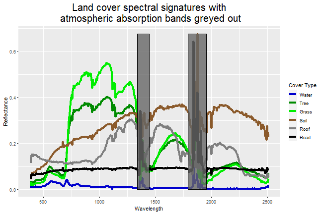
Now we can clearly see that the noisy sections of each spectral signature are within the atmospheric absorption bands. For our final step, let's take all reflectance values from within each absorption band and set them to NA to remove the noisiest sections from the plot.

# Duplicate the spectral signatures into a new data.frame

pixel.melt.masked <- pixel.melt

# Mask out all values within each of the two atmospheric absorption bands

pixel.melt.masked[pixel.melt.masked$wavelengths>ab1[1]&pixel.melt.masked$wavelengths<ab1[2],]$Reflectance <- NA

pixel.melt.masked[pixel.melt.masked$wavelengths>ab2[1]&pixel.melt.masked$wavelengths<ab2[2],]$Reflectance <- NA



# Plot the masked spectral signatures

ggplot()+
  geom_line(data = pixel.melt.masked, mapping = aes(x=wavelengths, y=Reflectance, color=variable), lwd=1.5)+
  scale_colour_manual(values = c("blue3","green4","green2","tan4","grey50","black"),
                      labels = c("Water","Tree","Grass","Soil","Roof","Road"))+
  labs(color = "Cover Type")+
  ggtitle("Land cover spectral signatures with\n atmospheric absorption bands removed")+
  theme(plot.title = element_text(hjust = 0.5, size=20))+
  xlab("Wavelength")

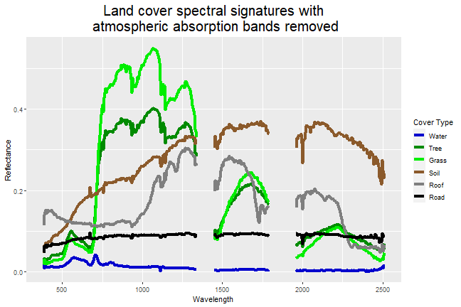
There you have it, spectral signatures for six different land cover types, with the regions from the atmospheric absorption bands removed.