Tutorial
The Relationship Between Raster Resolution, Spatial Extent & Number of Pixels
Last Updated: Apr 2, 2026
Learning Objectives:
After completing this activity, you will be able to:
- Explain the key attributes required to work with raster data including: spatial extent, coordinate reference system and spatial resolution.
- Describe what a spatial extent is and how it relates to resolution.
- Explain the basics of coordinate reference systems.
Things You’ll Need To Complete This Tutorial
You will need the most current version of R and, preferably, RStudio loaded
on your computer to complete this tutorial.
Install R Packages
-
raster:
install.packages("raster") -
rgdal:
install.packages("rgdal")
Data to Download
NEON Teaching Data Subset: Field Site Spatial Data
These remote sensing data files provide information on the vegetation at the National Ecological Observatory Network's San Joaquin Experimental Range and Soaproot Saddle field sites. The entire dataset can be accessed by request from the NEON Data Portal.
Download DatasetThe LiDAR and imagery data used to create the rasters in this dataset were collected over the San Joaquin field site located in California (NEON Domain 17) and processed at NEON headquarters. The entire dataset can be accessed by request from the NEON website.
This data download contains several files used in related tutorials. The path to
the files we will be using in this tutorial is:
NEON-DS-Field-Site-Spatial-Data/SJER/.
You should set your working directory to the parent directory of the downloaded
data to follow the code exactly.
This tutorial will overview the key attributes of a raster object, including
spatial extent, resolution and coordinate reference system. When working within
a GIS system often these attributes are accounted for. However, it is important
to be more familiar with them when working in non-GUI environments such as
R or even Python.
In order to correctly spatially reference a raster that is not already georeferenced, you will also need to identify:
- The lower left hand corner coordinates of the raster.
- The number of columns and rows that the raster dataset contains.
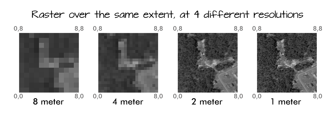
Spatial Resolution
A raster consists of a series of pixels, each with the same dimensions and shape. In the case of rasters derived from airborne sensors, each pixel represents an area of space on the Earth's surface. The size of the area on the surface that each pixel covers is known as the spatial resolution of the image. For instance, an image that has a 1 m spatial resolution means that each pixel in the image represents a 1 m x 1 m area.
Load the Data
Let's open up a raster in R to see how the attributes are stored. We are going to work with a Digital Terrain Model from the San Joaquin Experimental Range in California.
# load packages
library(raster)
library(rgdal)

# set working directory to data folder
#setwd("pathToDirHere")
wd <- ("~/Git/data/")
setwd(wd)

# Load raster in an R object called 'DEM'
DEM <- raster(paste0(wd, "NEON-DS-Field-Site-Spatial-Data/SJER/DigitalTerrainModel/SJER2013_DTM.tif"))


# View raster attributes
DEM

## class      : RasterLayer
## dimensions : 5060, 4299, 21752940  (nrow, ncol, ncell)
## resolution : 1, 1  (x, y)
## extent     : 254570, 258869, 4107302, 4112362  (xmin, xmax, ymin, ymax)
## crs        : +proj=utm +zone=11 +datum=WGS84 +units=m +no_defs
## source     : /Users/olearyd/Git/data/NEON-DS-Field-Site-Spatial-Data/SJER/DigitalTerrainModel/SJER2013_DTM.tif
## names      : SJER2013_DTM
Note that this raster (in GeoTIFF format) already has an extent, resolution, and CRS defined. The resolution in both x and y directions is 1. The CRS tells us that the x,y units of the data are meters (m).
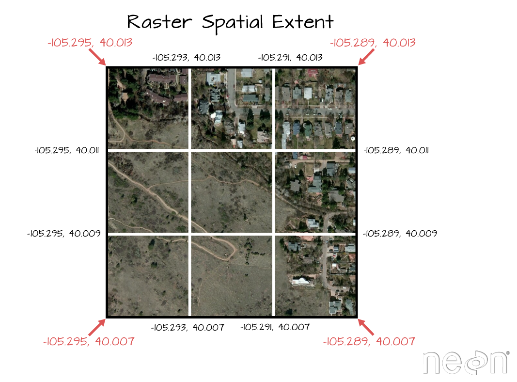
Spatial Extent
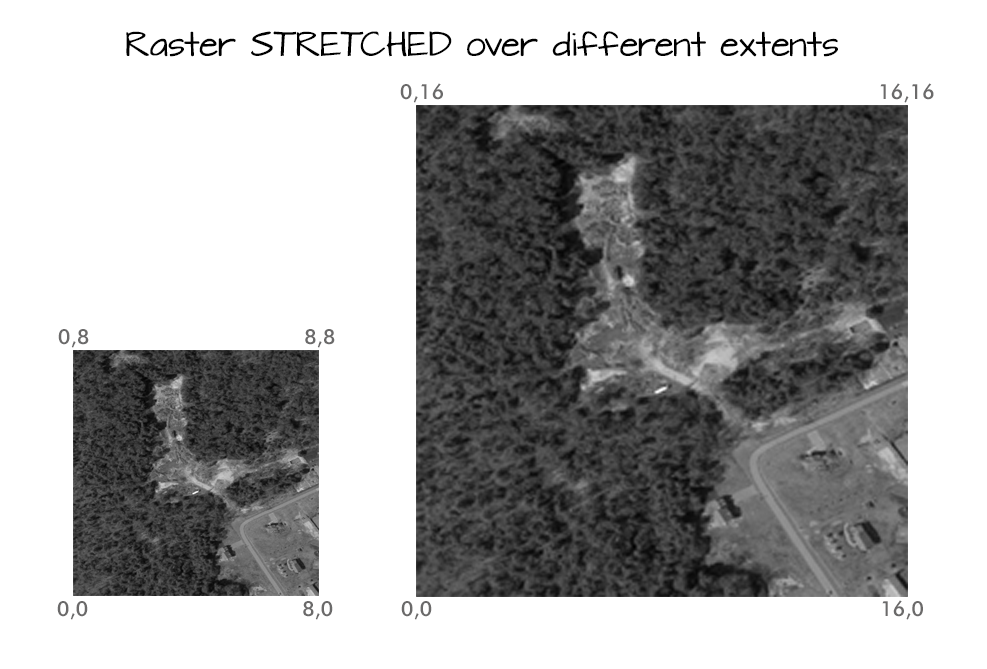
The spatial extent of a raster, represents the "X, Y" coordinates of the corners
of the raster in geographic space. This information, in addition to the cell
size or spatial resolution, tells the program how to place or render each pixel
in 2 dimensional space. Tools like R, using supporting packages such as rgdal
and associated raster tools have functions that allow you to view and define the
extent of a new raster.
# View the extent of the raster
DEM@extent

## class      : Extent
## xmin       : 254570
## xmax       : 258869
## ymin       : 4107302
## ymax       : 4112362
Calculating Raster Extent
Extent and spatial resolution are closely connected. To calculate the extent of a raster, we first need the bottom left hand (X,Y) coordinate of the raster. In the case of the UTM coordinate system which is in meters, to calculate the raster's extent, we can add the number of columns and rows to the X,Y corner coordinate location of the raster, multiplied by the resolution (the pixel size) of the raster.
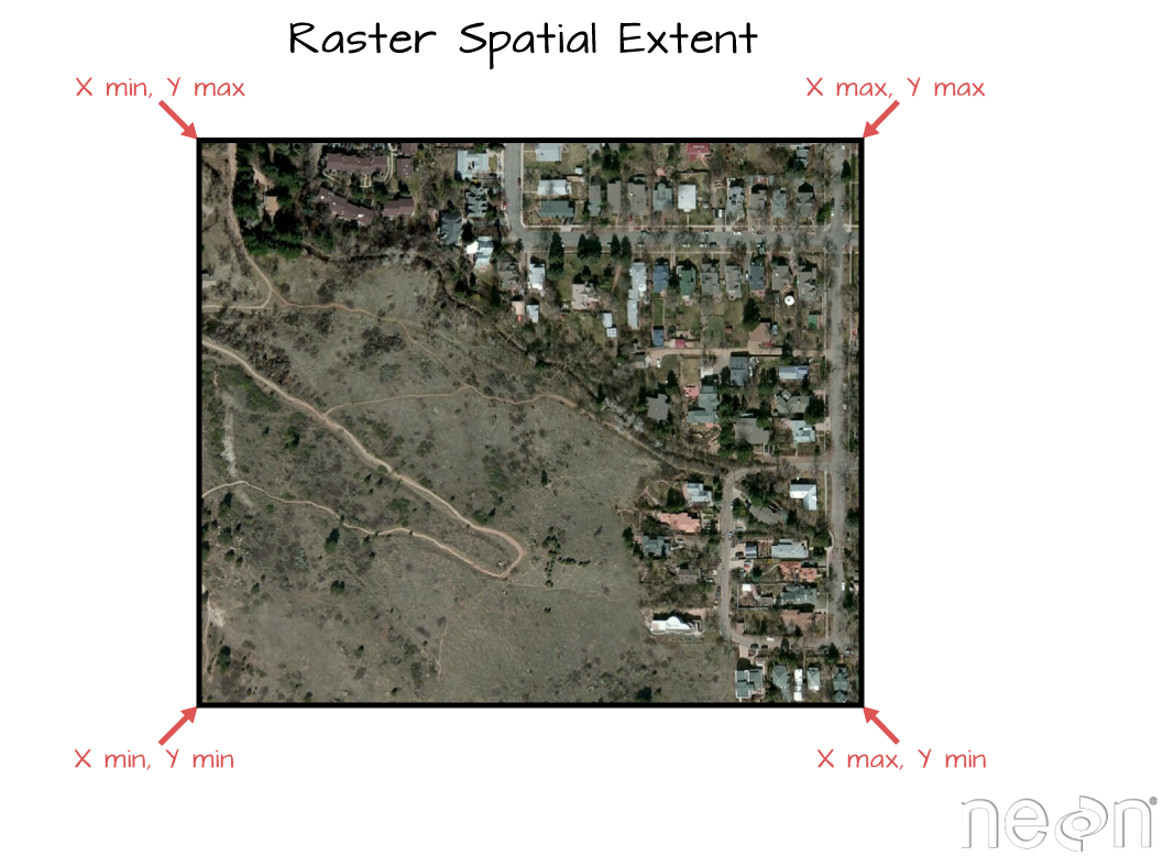
<figcaption>To be located geographically, a raster's location needs to be
defined in geographic space (i.e., on a spatial grid). The spatial extent
defines the four corners of a raster within a given coordinate reference
system. Source: National Ecological Observatory Network. </figcaption>
Let's explore that next, using a blank raster that we create.
# create a raster from the matrix - a "blank" raster of 4x4
myRaster1 <- raster(nrow=4, ncol=4)

# assign "data" to raster: 1 to n based on the number of cells in the raster
myRaster1[]<- 1:ncell(myRaster1)

# view attributes of the raster
myRaster1

## class      : RasterLayer
## dimensions : 4, 4, 16  (nrow, ncol, ncell)
## resolution : 90, 45  (x, y)
## extent     : -180, 180, -90, 90  (xmin, xmax, ymin, ymax)
## crs        : +proj=longlat +datum=WGS84 +no_defs
## source     : memory
## names      : layer
## values     : 1, 16  (min, max)

# is the CRS defined?
myRaster1@crs

## CRS arguments: +proj=longlat +datum=WGS84 +no_defs
Wait, why is the CRS defined on this new raster? This is the default values
for something created with the raster() function if nothing is defined.
Let's get back to looking at more attributes.
# what is the raster extent?
myRaster1@extent

## class      : Extent
## xmin       : -180
## xmax       : 180
## ymin       : -90
## ymax       : 90

# plot raster
plot(myRaster1, main="Raster with 16 pixels")
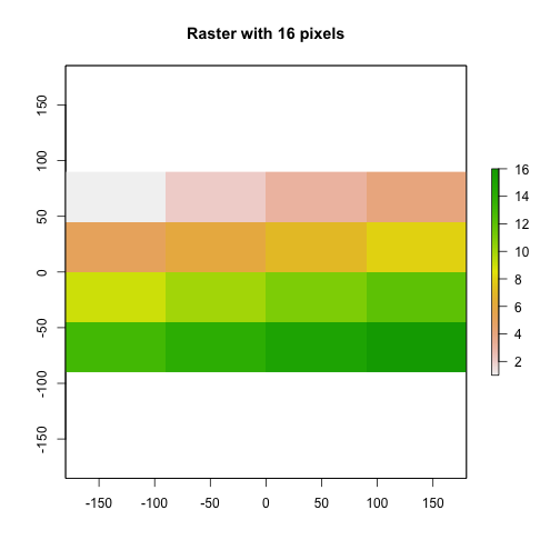
Here we see our raster with the value of 1 to 16 in each pixel.
We can resample the raster as well to adjust the resolution. If we want a higher resolution raster, we will apply a grid with more pixels within the same extent. If we want a lower resolution raster, we will apply a grid with fewer pixels within the same extent.
One way to do this is to create a raster of the resolution you want and then
resample() your original raster. The resampling will be done for either
nearest neighbor assignments (for categorical data) or bilinear interpolation (for
numerical data).
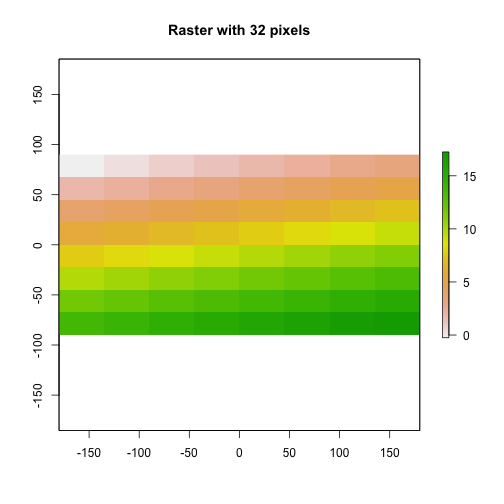
## HIGHER RESOLUTION
# Create 32 pixel raster
myRaster2 <- raster(nrow=8, ncol=8)

# resample 16 pix raster with 32 pix raster
# use bilinear interpolation with our numeric data
myRaster2 <- resample(myRaster1, myRaster2, method='bilinear')

# notice new dimensions, resolution, & min/max
myRaster2

## class      : RasterLayer
## dimensions : 8, 8, 64  (nrow, ncol, ncell)
## resolution : 45, 22.5  (x, y)
## extent     : -180, 180, -90, 90  (xmin, xmax, ymin, ymax)
## crs        : +proj=longlat +datum=WGS84 +no_defs
## source     : memory
## names      : layer
## values     : -0.25, 17.25  (min, max)

# plot
plot(myRaster2, main="Raster with 32 pixels")
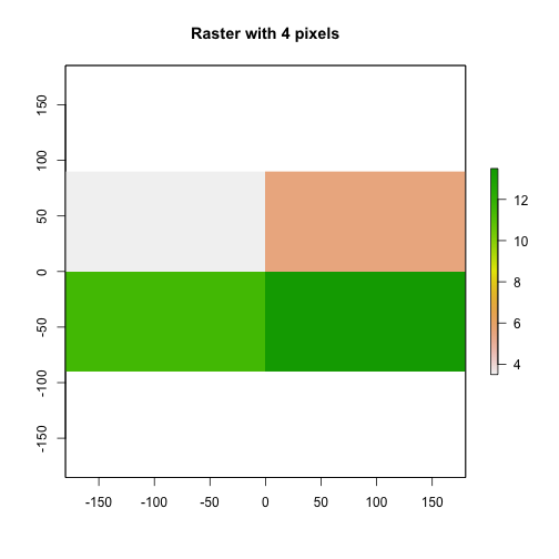
## LOWER RESOLUTION
myRaster3 <- raster(nrow=2, ncol=2)
myRaster3 <- resample(myRaster1, myRaster3, method='bilinear')
myRaster3

## class      : RasterLayer
## dimensions : 2, 2, 4  (nrow, ncol, ncell)
## resolution : 180, 90  (x, y)
## extent     : -180, 180, -90, 90  (xmin, xmax, ymin, ymax)
## crs        : +proj=longlat +datum=WGS84 +no_defs
## source     : memory
## names      : layer
## values     : 3.5, 13.5  (min, max)

plot(myRaster3, main="Raster with 4 pixels")
## SINGLE PIXEL RASTER
myRaster4 <- raster(nrow=1, ncol=1)
myRaster4 <- resample(myRaster1, myRaster4, method='bilinear')
myRaster4

## class      : RasterLayer
## dimensions : 1, 1, 1  (nrow, ncol, ncell)
## resolution : 360, 180  (x, y)
## extent     : -180, 180, -90, 90  (xmin, xmax, ymin, ymax)
## crs        : +proj=longlat +datum=WGS84 +no_defs
## source     : memory
## names      : layer
## values     : 7.666667, 7.666667  (min, max)

plot(myRaster4, main="Raster with 1 pixel")
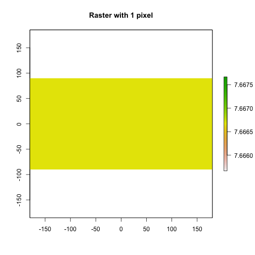
To more easily compare them, let's create a graphic layout with 4 rasters in it. Notice that each raster has the same extent but each a different resolution because it has a different number of pixels spread out over the same extent.
# change graphical parameter to 2x2 grid
par(mfrow=c(2,2))

# arrange plots in order you wish to see them
plot(myRaster2, main="Raster with 32 pixels")
plot(myRaster1, main="Raster with 16 pixels")
plot(myRaster3, main="Raster with 4 pixels")
plot(myRaster4, main="Raster with 2 pixels")
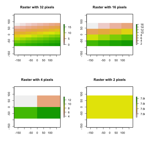
# change graphical parameter back to 1x1
par(mfrow=c(1,1))
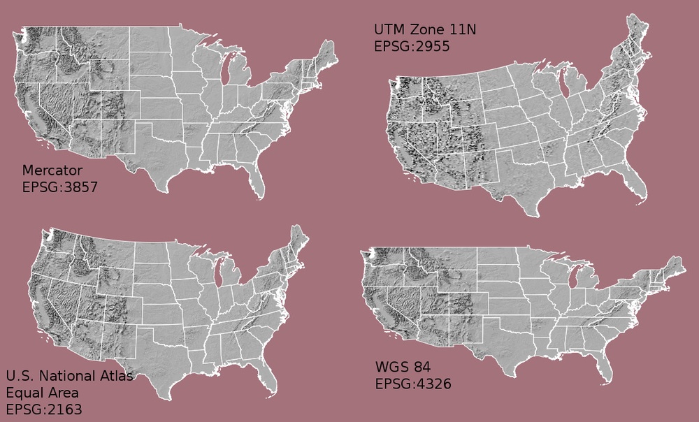
Extent & Coordinate Reference Systems
Coordinate Reference System & Projection Information
A spatial reference system (SRS) or coordinate reference system (CRS) is a coordinate-based local, regional or global system used to locate geographical entities. -- Wikipedia
The earth is round. This is not an new concept by any means, however we need to remember this when we talk about coordinate reference systems associated with spatial data. When we make maps on paper or on a computer screen, we are moving from a 3 dimensional space (the globe) to 2 dimensions (our computer screens or a piece of paper). To keep this short, the projection of a dataset relates to how the data are "flattened" in geographic space so our human eyes and brains can make sense of the information in 2 dimensions.
The projection refers to the mathematical calculations performed to "flatten the data" in into 2D space. The coordinate system references to the x and y coordinate space that is associated with the projection used to flatten the data. If you have the same dataset saved in two different projections, these two files won't line up correctly when rendered together.
How Map Projections Can Fool the Eye
Check out this short video, by Buzzfeed, highlighting how map projections can make continents seems proportionally larger or smaller than they actually are!
What Makes Spatial Data Line Up On A Map?
There are lots of great resources that describe coordinate reference systems and
projections in greater detail. However, for the purposes of this activity, what
is important to understand is that data from the same location but saved in
different projections will not line up in any GIS or other program. Thus
it's important when working with spatial data in a program like R or Python
to identify the coordinate reference system applied to the data, and to grab
that information and retain it when you process / analyze the data.
For a library of CRS information: A great online library of CRS information.
CRS proj4 Strings
The rgdal package has all the common ESPG codes with proj4string built in. We
can see them by creating an object of the function make_ESPG().
# make sure you loaded rgdal package at the top of your script

# create an object with all ESPG codes
epsg = make_EPSG()

# use View(espg) to see the full table - doesn't render on website well
#View(epsg)

# View top 5 entries
head(epsg, 5)

##   code   note                                                   prj4
## 1 3819 HD1909         +proj=longlat +ellps=bessel +no_defs +type=crs
## 2 3821  TWD67        +proj=longlat +ellps=aust_SA +no_defs +type=crs
## 3 3822  TWD97 +proj=geocent +ellps=GRS80 +units=m +no_defs +type=crs
## 4 3823  TWD97          +proj=longlat +ellps=GRS80 +no_defs +type=crs
## 5 3824  TWD97          +proj=longlat +ellps=GRS80 +no_defs +type=crs
##   prj_method
## 1     (null)
## 2     (null)
## 3     (null)
## 4     (null)
## 5     (null)
Define the extent
In the above raster example, we created several simple raster objects in R. R defaulted to a global lat/long extent. We can define the exact extent that we need to use too.
Let's create a new raster with the same projection as our original DEM. We know that our data are in UTM zone 11N. For the sake of this exercise, let say we want to create a raster with the left hand corner coordinate at:
- xmin = 254570
- ymin = 4107302
The resolution of this new raster will be 1 meter and we will be working
in UTM (meters). First, let's set up the raster.
# create 10x20 matrix with values 1-8.
newMatrix  <- (matrix(1:8, nrow = 10, ncol = 20))

# convert to raster
rasterNoProj <- raster(newMatrix)
rasterNoProj

## class      : RasterLayer
## dimensions : 10, 20, 200  (nrow, ncol, ncell)
## resolution : 0.05, 0.1  (x, y)
## extent     : 0, 1, 0, 1  (xmin, xmax, ymin, ymax)
## crs        : NA
## source     : memory
## names      : layer
## values     : 1, 8  (min, max)
Now we can define the new raster's extent by defining the lower left corner of the raster.
## Define the xmin and ymin (the lower left hand corner of the raster)

# 1. define xMin & yMin objects.
xMin = 254570
yMin = 4107302

# 2. grab the cols and rows for the raster using @ncols and @nrows
rasterNoProj@ncols

## [1] 20

rasterNoProj@nrows

## [1] 10

# 3. raster resolution
res <- 1.0

# 4. add the numbers of cols and rows to the x,y corner location,
# result = we get the bounds of our raster extent.
xMax <- xMin + (rasterNoProj@ncols * res)
yMax <- yMin + (rasterNoProj@nrows * res)

# 5.create a raster extent class
rasExt <- extent(xMin,xMax,yMin,yMax)
rasExt

## class      : Extent
## xmin       : 254570
## xmax       : 254590
## ymin       : 4107302
## ymax       : 4107312

# 6. apply the extent to our raster
rasterNoProj@extent <- rasExt

# Did it work?
rasterNoProj

## class      : RasterLayer
## dimensions : 10, 20, 200  (nrow, ncol, ncell)
## resolution : 1, 1  (x, y)
## extent     : 254570, 254590, 4107302, 4107312  (xmin, xmax, ymin, ymax)
## crs        : NA
## source     : memory
## names      : layer
## values     : 1, 8  (min, max)

# or view extent only
rasterNoProj@extent

## class      : Extent
## xmin       : 254570
## xmax       : 254590
## ymin       : 4107302
## ymax       : 4107312
Now we have an extent associated with our raster which places it in space!
# plot new raster
plot(rasterNoProj, main="Raster in UTM coordinates, 1 m resolution")
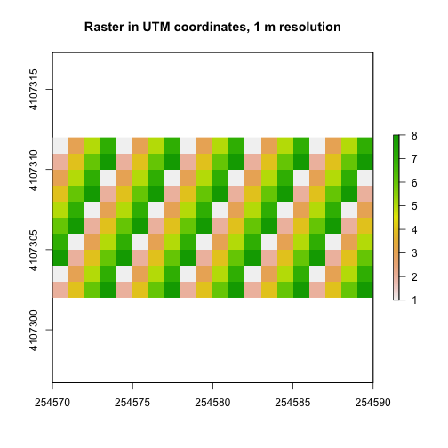
Notice that the coordinates show up on our plot now.
Now apply your skills in a new way!
- Resample
rasterNoProjfrom 1 meter to 10 meter resolution. Plot it next to the 1 m resolution raster. Use:par(mfrow=c(1,2))to create side by side plots. - What happens to the extent if you change the resolution to 1.5 when calculating the raster's extent properties??
Define Projection of a Raster
We can define the projection of a raster that has a known CRS already. Sometimes we download data that have projection information associated with them but the CRS is not defined either in the GeoTIFF tags or in the raster itself. If this is the case, we can simply assign the raster the correct projection.
Be careful doing this - it is not the same thing as reprojecting your data.
Let's define the projection for our newest raster using the DEM raster that already has defined CRS. NOTE: in this case we have to know that our raster is in this projection already so we don't run the risk of assigning the wrong projection to the data.
# view CRS from raster of interest
rasterNoProj@crs

## CRS arguments: NA

# view the CRS of our DEM object.
DEM@crs

## CRS arguments:
##  +proj=utm +zone=11 +datum=WGS84 +units=m +no_defs

# define the CRS using a CRS of another raster
rasterNoProj@crs <- DEM@crs

# look at the attributes
rasterNoProj

## class      : RasterLayer
## dimensions : 10, 20, 200  (nrow, ncol, ncell)
## resolution : 1, 1  (x, y)
## extent     : 254570, 254590, 4107302, 4107312  (xmin, xmax, ymin, ymax)
## crs        : +proj=utm +zone=11 +datum=WGS84 +units=m +no_defs
## source     : memory
## names      : layer
## values     : 1, 8  (min, max)

# view just the crs
rasterNoProj@crs

## CRS arguments:
##  +proj=utm +zone=11 +datum=WGS84 +units=m +no_defs
IMPORTANT: the above code does not reproject the raster. It simply defines the
Coordinate Reference System based upon the CRS of another raster. If you want to
actually change the CRS of a raster, you need to use the projectRaster function.
You can set the CRS and extent of a raster using the syntax
rasterWithoutReference@crs <- rasterWithReference@crs and
rasterWithoutReference@extent <- rasterWithReference@extent. Using this information:
- open
band90.tifin therasterLayers_tiffolder and plot it. (You could consider looking at it in QGIS first to compare it to the other rasters.) - Does it line up with our DEM? Look closely at the extent and pixel size. Does anything look off?
- Fix what is missing.
- (Advanced step) Export a new GeoTIFF Do things line up in QGIS?
The code below creates a raster and seeds it with some data. Experiment with the code.
- What happens to the resulting raster's resolution when you change the range of lat and long values to 5 instead of 10? Try 20, 50 and 100?
- What is the relationship between the extent and the raster resolution?
## Challenge Example Code

# set latLong
latLong <- data.frame(longitude=seq( 0,10,1), latitude=seq( 0,10,1))

# make spatial points dataframe, which will have a spatial extent
sp <- SpatialPoints( latLong[ c("longitude" , "latitude") ], proj4string = CRS("+proj=longlat +datum=WGS84") )

# make raster based on the extent of your data
r <- raster(nrow=5, ncol=5, extent( sp ) )

r[]  <- 1
r[]  <- sample(0:50,25)
r

## class      : RasterLayer
## dimensions : 5, 5, 25  (nrow, ncol, ncell)
## resolution : 2, 2  (x, y)
## extent     : 0, 10, 0, 10  (xmin, xmax, ymin, ymax)
## crs        : NA
## source     : memory
## names      : layer
## values     : 3, 50  (min, max)
Reprojecting Data
If you run into multiple spatial datasets with varying projections, you can always reproject the data so that they are all in the same projection. Python and R both have reprojection tools that perform this task.
# reproject raster data from UTM to CRS of Lat/Long WGS84
reprojectedData1 <- projectRaster(rasterNoProj,
                                 crs="+proj=longlat +ellps=WGS84 +datum=WGS84 +no_defs ")

# note that the extent has been adjusted to account for the NEW crs
reprojectedData1@crs

## CRS arguments: +proj=longlat +datum=WGS84 +no_defs

reprojectedData1@extent

## class      : Extent
## xmin       : -119.761
## xmax       : -119.7607
## ymin       : 37.07988
## ymax       : 37.08

# note the range of values in the output data
reprojectedData1

## class      : RasterLayer
## dimensions : 13, 22, 286  (nrow, ncol, ncell)
## resolution : 1.12e-05, 9e-06  (x, y)
## extent     : -119.761, -119.7607, 37.07988, 37.08  (xmin, xmax, ymin, ymax)
## crs        : +proj=longlat +datum=WGS84 +no_defs
## source     : memory
## names      : layer
## values     : 0.64765, 8.641957  (min, max)

# use nearest neighbor interpolation method to ensure that the values stay the same
reprojectedData2 <- projectRaster(rasterNoProj,
                                 crs="+proj=longlat +ellps=WGS84 +datum=WGS84 +no_defs ",
                                 method = "ngb")


# note that the min and max values have now been forced to stay within the same range.
reprojectedData2

## class      : RasterLayer
## dimensions : 13, 22, 286  (nrow, ncol, ncell)
## resolution : 1.12e-05, 9e-06  (x, y)
## extent     : -119.761, -119.7607, 37.07988, 37.08  (xmin, xmax, ymin, ymax)
## crs        : +proj=longlat +datum=WGS84 +no_defs
## source     : memory
## names      : layer
## values     : 1, 8  (min, max)