Tutorial
New Resources for Working with NEON Data
Last Updated: Jun 30, 2026
This tutorial provides a tour of recent (as of fall 2025, with a minor update in spring 2026) updates and enhancements to NEON code resources.
If you are new to using NEON data, we recommend first following the Download and Explore tutorial to get familiar with NEON data formats and the neonUtilities package.
Set up R environment
First install and load the necessary packages. As of June 2026, NEON requires an API token for data downloads, to reduce bot scraping and improve user support. Tokens can be generated in NEON data portal user accounts - log in to your account or create one, and go to the API Tokens section. For best practices in storing and using tokens, follow the instructions here.
# install packages. can skip this step if

# the packages are already installed

install.packages("neonUtilities")

install.packages("neonOS")

install.packages("lubridate")

install.packages("ggplot2")

install.packages("dplyr")

install.packages("visNetwork")


# load packages

library(neonUtilities)

library(neonOS)

library(ggplot2)

library(lubridate)

library(dplyr)

library(visNetwork)


token <- Sys.getenv("NEON_TOKEN")
The neonOS package
The neonOS package provides functions specifically for working with NEON observational (OS) data products. NEON's human-collected data present some unique challenges: the structure and data relationships within each product are unique, automation is more difficult, and sample relationships are often essential. The neonOS package contains functions for duplicate checking, table joining, and sample exploration.
For a detailed introduction to the neonOS package, see the full tutorial. Here we'll do a quick overview.
We'll use soil data throughout as an example dataset to illustrate code features. Let's say we're interested in the relationships between soil chemistry, microbial communities, and disturbance events. Start by downloading Soil physical and chemical properties, periodic (DP1.10086.001) from Soaproot Saddle (SOAP), 2018-2024.
Feature: Omit progress bars
Progress bars can now be suppressed in download functions in the neonUtilities package. This can be helpful when running code in an automated workflow or batch script. Note that messages associated with progress will be suppressed along with the bars, but messages about exceptions or errors will still be printed to the console.
soil <- loadByProduct(dpID="DP1.10086.001",
                     site="SOAP",
                     startdate="2018-01",
                     enddate="2024-12",
                     include.provisional=T,
                     progress=F,
                     check.size=F,
                     token=token)


list2env(soil, .GlobalEnv)
To start, we want to assess whether soil moisture is associated with different nitrogen content. Moisture data are in the sls_soilMoisture table, and nitrogen data are in the sls_soilChemistry table. We'll need to join the tables.
But before joining, let's check both tables for duplicates.
Feature: Check for duplicate records
moisturedups <- removeDups(sls_soilMoisture,
                           variables_10086)

## No duplicated key values found!

chemdups <- removeDups(sls_soilChemistry,
                       variables_10086)

## No duplicated key values found!
Neither table contains any duplicates. This is common - staff internal to NEON take advantage of these code resources, too, and use them to detect and resolve duplicates. However, especially if you use Provisional data, it's a good idea to check. See the neonOS tutorial for more details about the removeDups() function, and to see an example that does contain duplicates.
Now we can join the tables.
Feature: Join observational data tables
moistchem <- joinTableNEON(moisturedups,
                           chemdups,
                           name1="sls_soilMoisture",
                           name2="sls_soilChemistry")
Now that we have the nitrogen and moisture data in a single table, we can compare.
plot(nitrogenPercent~soilMoisture,
     data=moistchem,
     pch=20)
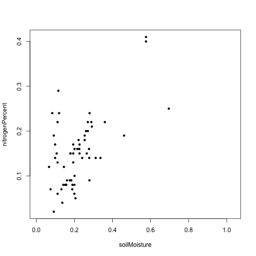
Within this dataset, wetter soils tend to also be higher in nitrogen.
Event data
We are also interested in the impact of disturbance on these soils. Soaproot Saddle is in California - has it burned during the observed time period?
The Site management and event reporting (DP1.10111.001) data product contains records of disturbance and management events that occur at NEON sites. We could download all records from SOAP, but a new function in neonUtilities allows us to run a targeted query for specific event types.
Feature: Get event data by event type
sim <- byEventSIM("fire",
                  site="SOAP",
                  token=token)


sim$sim_eventData

##                                    uid domainID siteID namedLocation
## 1 2c8c0bf8-caf0-4c48-bad3-590d0e737047      D17   SOAP          SOAP
## 2 0c1fcf9f-5bee-478c-8412-0bf57925a04b      D17   SOAP          SOAP
## 3 4ffe7ac8-ff68-48e8-97e6-2efd446cd3da      D17   SOAP          SOAP
## 4 53b0b814-8441-41c4-a44b-91fc3413d97b      D17   SOAP          SOAP
## 5 6b641a93-0494-4998-9d8a-c56df5d70891      D17   SOAP          SOAP
## 6 8bc10c21-79b3-4421-b0ae-703f98067e6f      D17   SOAP          SOAP
##                                                                                                                                                                                                                                                                                                                                                                                                                                                                                                                                                                                                                                                                                                                                                                                                                                                                                                 locationID
## 1                                                                                                                                                                                                                                                                                                                                                                                                                                                                                                                                                                                                                                                                             SOAP_007.basePlot.all, SOAP_016.basePlot.all, SOAP_017.basePlot.all, SOAP_018.basePlot.all, SOAP_019.basePlot.all, SOAP_003.tickPlot.tck, SOAP_036.mosquitoPoint.mos, SOAP_039.mosquitoPoint.mos, SOAP_041.mosquitoPoint.mos
## 2 SOAP_002.basePlot.all, SOAP_005.basePlot.all, SOAP_006.basePlot.all, SOAP_008.basePlot.all, SOAP_012.basePlot.all, SOAP_013.basePlot.all, SOAP_023.basePlot.all, SOAP_024.basePlot.all, SOAP_026.basePlot.all, SOAP_027.basePlot.all, SOAP_028.basePlot.all, SOAP_043.basePlot.all, SOAP_044.basePlot.all, SOAP_046.basePlot.all, SOAP_050.basePlot.all, SOAP_051.basePlot.all, SOAP_052.basePlot.all, SOAP_055.basePlot.all, SOAP_058.basePlot.all, SOAP_059.basePlot.all, SOAP_060.basePlot.all, SOAP_061.basePlot.all, SOAP_005.tickPlot.tck, SOAP_006.tickPlot.tck, SOAP_026.tickPlot.tck, SOAP_002.mammalGrid.mam, SOAP_006.mammalGrid.mam, SOAP_008.mammalGrid.mam, SOAP_012.mammalGrid.mam, SOAP_032.mammalGrid.mam, SOAP_033.mosquitoPoint.mos, SOAP_035.mosquitoPoint.mos, SOAP_037.mosquitoPoint.mos, SOAP_038.mosquitoPoint.mos, SOAP_039.mosquitoPoint.mos, SOAP_040.mosquitoPoint.mos, SOAP
## 3 SOAP_002.basePlot.all, SOAP_005.basePlot.all, SOAP_006.basePlot.all, SOAP_008.basePlot.all, SOAP_012.basePlot.all, SOAP_013.basePlot.all, SOAP_023.basePlot.all, SOAP_024.basePlot.all, SOAP_026.basePlot.all, SOAP_027.basePlot.all, SOAP_028.basePlot.all, SOAP_043.basePlot.all, SOAP_044.basePlot.all, SOAP_046.basePlot.all, SOAP_050.basePlot.all, SOAP_051.basePlot.all, SOAP_052.basePlot.all, SOAP_055.basePlot.all, SOAP_058.basePlot.all, SOAP_059.basePlot.all, SOAP_060.basePlot.all, SOAP_061.basePlot.all, SOAP_005.tickPlot.tck, SOAP_006.tickPlot.tck, SOAP_026.tickPlot.tck, SOAP_002.mammalGrid.mam, SOAP_006.mammalGrid.mam, SOAP_008.mammalGrid.mam, SOAP_012.mammalGrid.mam, SOAP_032.mammalGrid.mam, SOAP_033.mosquitoPoint.mos, SOAP_035.mosquitoPoint.mos, SOAP_037.mosquitoPoint.mos, SOAP_038.mosquitoPoint.mos, SOAP_039.mosquitoPoint.mos, SOAP_040.mosquitoPoint.mos, SOAP
## 4 SOAP_002.basePlot.all, SOAP_005.basePlot.all, SOAP_006.basePlot.all, SOAP_008.basePlot.all, SOAP_012.basePlot.all, SOAP_013.basePlot.all, SOAP_023.basePlot.all, SOAP_024.basePlot.all, SOAP_026.basePlot.all, SOAP_027.basePlot.all, SOAP_028.basePlot.all, SOAP_043.basePlot.all, SOAP_044.basePlot.all, SOAP_046.basePlot.all, SOAP_050.basePlot.all, SOAP_051.basePlot.all, SOAP_052.basePlot.all, SOAP_055.basePlot.all, SOAP_058.basePlot.all, SOAP_059.basePlot.all, SOAP_060.basePlot.all, SOAP_061.basePlot.all, SOAP_005.tickPlot.tck, SOAP_006.tickPlot.tck, SOAP_026.tickPlot.tck, SOAP_002.mammalGrid.mam, SOAP_006.mammalGrid.mam, SOAP_008.mammalGrid.mam, SOAP_012.mammalGrid.mam, SOAP_032.mammalGrid.mam, SOAP_033.mosquitoPoint.mos, SOAP_035.mosquitoPoint.mos, SOAP_037.mosquitoPoint.mos, SOAP_038.mosquitoPoint.mos, SOAP_039.mosquitoPoint.mos, SOAP_040.mosquitoPoint.mos, SOAP
## 5 SOAP_002.basePlot.all, SOAP_005.basePlot.all, SOAP_006.basePlot.all, SOAP_008.basePlot.all, SOAP_012.basePlot.all, SOAP_013.basePlot.all, SOAP_023.basePlot.all, SOAP_024.basePlot.all, SOAP_026.basePlot.all, SOAP_027.basePlot.all, SOAP_028.basePlot.all, SOAP_043.basePlot.all, SOAP_044.basePlot.all, SOAP_046.basePlot.all, SOAP_050.basePlot.all, SOAP_051.basePlot.all, SOAP_052.basePlot.all, SOAP_055.basePlot.all, SOAP_058.basePlot.all, SOAP_059.basePlot.all, SOAP_060.basePlot.all, SOAP_061.basePlot.all, SOAP_005.tickPlot.tck, SOAP_006.tickPlot.tck, SOAP_026.tickPlot.tck, SOAP_002.mammalGrid.mam, SOAP_006.mammalGrid.mam, SOAP_008.mammalGrid.mam, SOAP_012.mammalGrid.mam, SOAP_032.mammalGrid.mam, SOAP_033.mosquitoPoint.mos, SOAP_035.mosquitoPoint.mos, SOAP_037.mosquitoPoint.mos, SOAP_038.mosquitoPoint.mos, SOAP_039.mosquitoPoint.mos, SOAP_040.mosquitoPoint.mos, SOAP
## 6                                                                                                                                                                                                                                                                                                                                                                                                                                                                                                                                                                                                                                                                                     SOAP_014.basePlot.all, SOAP_016.basePlot.all, SOAP_020.basePlot.all, SOAP_045.basePlot.all, SOAP_047.basePlot.all, SOAP_053.basePlot.all, SOAP_054.basePlot.all, SOAP_056.basePlot.all, SOAP_062.phenology.phe, SOAP
##    startDate    endDate ongoingEvent estimatedOrActualDate dateRemarks            eventID samplingProtocolVersion eventType
## 1 2020-02-24 2020-03-09            N                  <NA>        <NA> SOAP.20200224.fire       NEON.DOC.003282vC      fire
## 2 2020-09-04 2020-10-04            Y                actual        <NA> SOAP.20200904.fire       NEON.DOC.003282vD      fire
## 3 2020-10-04 2020-11-03            Y                actual        <NA> SOAP.20201004.fire       NEON.DOC.003282vD      fire
## 4 2020-11-03 2020-12-03            Y                actual        <NA> SOAP.20201004.fire       NEON.DOC.003282vD      fire
## 5 2020-12-03 2020-12-24            N                actual        <NA> SOAP.20201004.fire       NEON.DOC.003282vD      fire
## 6 2021-06-29 2021-07-08            N                actual        <NA> SOAP.20210629.fire       NEON.DOC.003282vD      fire
##      methodTypeChoice name scientificName otherScientificName fireSeverity biomassRemoval minQuantity maxQuantity
## 1 fire-controlledBurn <NA>           <NA>                <NA>      unknown           <NA>          NA          NA
## 2       fire-wildfire <NA>           <NA>                <NA>         high           <NA>          NA          NA
## 3       fire-wildfire <NA>           <NA>                <NA>         high           <NA>          NA          NA
## 4       fire-wildfire <NA>           <NA>                <NA>         high           <NA>          NA          NA
## 5       fire-wildfire <NA>           <NA>                <NA>         high           <NA>          NA          NA
## 6       fire-wildfire <NA>           <NA>                <NA>         high           <NA>          NA          NA
##   quantityUnit reporterType         remarks          recordedBy dataQF
## 1         <NA>    secondary controlled burn 0000-0002-4748-8985   <NA>
## 2         <NA>      primary      Creek Fire 0000-0001-7920-7757   <NA>
## 3         <NA>      primary      Creek Fire 0000-0001-7920-7757   <NA>
## 4         <NA>      primary      Creek Fire 0000-0001-7920-7757   <NA>
## 5         <NA>      primary      Creek Fire 0000-0001-7920-7757   <NA>
## 6         <NA>      primary       Blue Fire 0000-0001-7920-7757   <NA>
##                                                                                                                                                                                               filename
## 1 https://storage.googleapis.com/neon-publication/NEON.DOM.SITE.DP1.10111.001/SOAP/20200301T000000--20200401T000000/basic/NEON.D17.SOAP.DP1.10111.001.sim_eventData.2020-03.basic.20251205T223131Z.csv
## 2 https://storage.googleapis.com/neon-publication/NEON.DOM.SITE.DP1.10111.001/SOAP/20201001T000000--20201101T000000/basic/NEON.D17.SOAP.DP1.10111.001.sim_eventData.2020-10.basic.20251205T212610Z.csv
## 3 https://storage.googleapis.com/neon-publication/NEON.DOM.SITE.DP1.10111.001/SOAP/20201101T000000--20201201T000000/basic/NEON.D17.SOAP.DP1.10111.001.sim_eventData.2020-11.basic.20251205T220607Z.csv
## 4 https://storage.googleapis.com/neon-publication/NEON.DOM.SITE.DP1.10111.001/SOAP/20201201T000000--20210101T000000/basic/NEON.D17.SOAP.DP1.10111.001.sim_eventData.2020-12.basic.20251205T213421Z.csv
## 5 https://storage.googleapis.com/neon-publication/NEON.DOM.SITE.DP1.10111.001/SOAP/20201201T000000--20210101T000000/basic/NEON.D17.SOAP.DP1.10111.001.sim_eventData.2020-12.basic.20251205T213421Z.csv
## 6 https://storage.googleapis.com/neon-publication/NEON.DOM.SITE.DP1.10111.001/SOAP/20210701T000000--20210801T000000/basic/NEON.D17.SOAP.DP1.10111.001.sim_eventData.2021-07.basic.20251206T022332Z.csv
There are six records about fires at SOAP. Looking at the details, we can see one controlled burn in 2020, the Creek Fire in 2020 (four records), and the Blue Fire in 2021.
How does this compare to the measurement dates for the chemistry data?
unique(year(sls_soilChemistry$collectDate))

## [1] 2018 2024
Chemistry measurements were made in 2018 and 2024, before and after the fires. Do nitrogen values differ between the two measurement dates?
plot(nitrogenPercent~soilMoisture,
     data=subset(moistchem,
                 year(collectDate.y)==2018),
     pch=20)

points(nitrogenPercent~soilMoisture,
     data=subset(moistchem,
                 year(collectDate.y)==2024),
     pch=20, col="red")
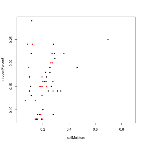
No obvious differences in the pattern between the two measurement dates.
If we wanted to dig into the effects of fire more deeply, note that the event data table includes a locationID field. This field contains a record of the NEON sampling plots affected by the event - in this case, which plots burned. If there are both burned and unburned plots in our dataset, this could be very informative.
Site management location data details
There is a new NEON code package to help users to more easily work with the location data associated with site events. Get an introduction to this package in the Site management tutorial.
Community data
We mentioned above that we are also interested in microbial communities. What microbes are living in these soils, and how have they changed over time? Let's download the Soil microbe community taxonomy (DP1.10081.002) data for the same time period at SOAP.
Feature: Seamless stacking of microbe community data
The community data are in the expanded data package.
micro <- loadByProduct(dpID="DP1.10081.002",
                     site="SOAP",
                     startdate="2018-05",
                     enddate="2024-12",
                     package="expanded",
                     include.provisional=T,
                     progress=F,
                     check.size=F,
                     token=token)

## Stacking per-sample files. These files may be very large; download data in smaller subsets if performance problems are encountered.

list2env(micro, .GlobalEnv)
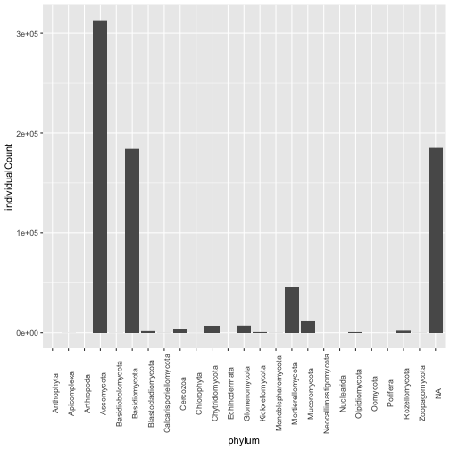
Let's look at the distribution by phylum of fungal taxon units at SOAP.
gg <- ggplot(mct_soilPerSampleTaxonomy_ITS,
             aes(phylum, individualCount)) +
  geom_col() +
  theme(axis.text.x = element_text(angle = 90))

gg
But can we compare the communities at the two time points?
unique(year(mct_soilSampleMetadata_ITS$collectDate))

## [1] 2018 2024
Marker gene data were collected in 2024, but the community taxonomy data are not available yet.
Suppose we wanted to compare soil chemistry data to plant communities instead of microbial communities? The Plant presence and percent cover (DP1.10058.001) data product would be a good place to start.
Pending feature: neonPlants R package
We are very close to releasing the neonPlants package, which will facilitate use of NEON's various plant data products, including both community and biomass data. Stay tuned!
Samples
We've seen above that not all soil samples have associated microbial data. Is there an efficient way to find out the downstream samples from a specific sample?
The neonOS package includes a function to find the complete sample hierarchy for any given sample. This can be helpful for understanding sample relationships and for interfacing with the NEON Biorepository.
Feature: Get sample hierarchies
Let's look at the sample hierarchies from the first two soil samples in the dataset we downloaded. We'll use the visNetwork package (a public package not specific to NEON) to visualize the sample relationships.
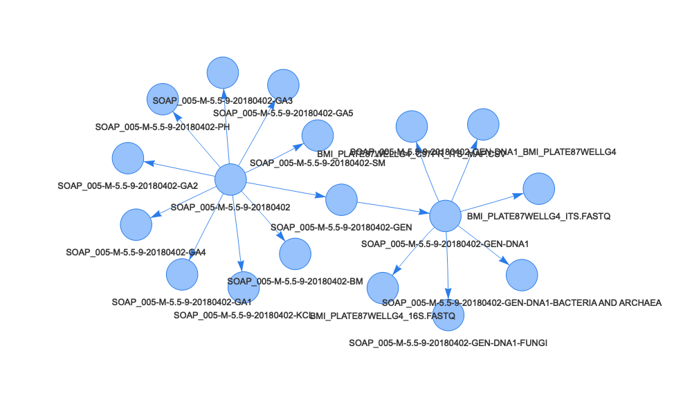
First sample:
samp <- getSampleTree(sls_soilCoreCollection$sampleID[1],
                      token=token)

edges <- data.frame(cbind(to=samp$sampleUuid,
                          from=samp$parentSampleUuid))

nodes <- data.frame(cbind(id=samp$sampleUuid,
                          label=samp$sampleTag))

visNetwork(nodes, edges) |>
  visEdges(arrows="to")
Second sample:
samp <- getSampleTree(sls_soilCoreCollection$sampleID[2],
                      token=token)

edges <- data.frame(cbind(to=samp$sampleUuid,
                          from=samp$parentSampleUuid))

nodes <- data.frame(cbind(id=samp$sampleUuid,
                          label=samp$sampleTag))

visNetwork(nodes, edges) |>
  visEdges(arrows="to")
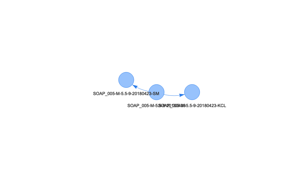
We can see the second sample tree is much simpler than the first - the soil core has two child samples, a soil moisture and a KCl extract sample. The first sample produced many subsamples, for moisture, pH, genetic archive, and sequencing, and the sequencing sample produced six subsamples of its own.
Because you can only query one sample at a time this way, its capabilities to support analyses are limited. But it can be very helpful in understanding NEON's sample workflows and processes. And if you're working with Biorepository samples, you can use this to find the upstream samples from an archived sample. Your query can start with any sample in the hierarchy, it doesn't have to start at the top.
Other languages and platforms
Feature: Python version of neonutilities
For years, neonUtilities has only been available in R, but as of 2024 we have a Python version!
Aside from some minor formatting differences - neonutilities in all lower case, function names in snake_case rather than camelCase - the functions and inputs are the same in Python as in R. For example, to download the same soil dataset:
import neonutilities as nu
dotenv.load_dotenv()
token = os.environ.get("NEON_TOKEN")

soil = nu.load_by_product(dpid="DP1.10086.001",
                     site="SOAP",
                     startdate="2018-01",
                     enddate="2024-12",
                     include_provisional=True,
                     progress=False,
                     check_size=False,
                     token=token)
Other code packages, including neonOS and geoNEON, haven't been implemented in Python yet.
Feature: Surface-atmosphere exchange data stacking in Python
This is now available in the stack_eddy() function! The Introduction to NEON Flux Data tutorial now includes code in both languages.
Feature: Cloud mode
The loadByProduct() function works by downloading NEON data files to a temporary directory and then reading them into R in stacked form. With new cloud-native software, it is possible to accomplish this without the intermediate download step - the files are imported directly to the code environment and stacked simultaneously. If you are working in a cloud environment, add the input cloud.mode=T (or cloud_mode=True in Python) to loadByProduct() for much faster and more efficient data access.
If you are new to working in cloud environments but want to start exploring, we recommend checking out CyVerse.
Stay connected!
New code releases and updates are announced via NEON data notifications. Sign up to get data notifications sent to your inbox by making a NEON user account.
If you have any questions, or want to request new features, use the Contact Us page.