Tutorial
Exploring sample availability at the NEON Biorepository
Last Updated: Jun 30, 2026
Learning Objectives
In this tutorial, we will learn how to develop a sample list to optimally answer a research question based on NEON data product and NEON Biorepository sample availability.
-
Outline a broad research question.
-
Download related data from the main NEON data portal using the
neonUtilitiesR package. -
Compare NEON data availability across multiple data products in order to narrow research scope.
-
Identify NEON Biorepository samples that match the research scope of interest using NEON Biorepository data.
-
Visualize our request in an interactive map.
Research question
We are interested in testing for relationships between the diet of small mammals and the carbon and nitrogen stable isotope ratios in co-occurring plant communities in a portion of the eastern United States. NEON provides extensive information about stable isotopes from samples collected from the canopy and in litter traps. While NEON does not measure small mammal diets as part of its focal protocols, NEON archives both hair and fecal samples that researchers can use to gain these insights.
What samples from the NEON Biorepository can be requested in order to conduct this study?
To answer this this question, we need to understand where there is spatial and temporal overlap in measurements of canopy foliar chemistry, litter chemistry, and mammal sampling.
We will attempt to develop a list of samples following these criteria:
-
Site and year combinations for which carbon nitrogen ratio measurements are available for both canopy foliage and litter
-
Common species for which we can achieve a minimum viable sample size for our study
-
Both a hair and a fecal sample were collected from the same individual
Background information on the NEON Biorepository
The NEON Biorepository is located at Arizona State University and serves as the primary repository for the 100,000 NEON samples and specimens collected across all 81 NEON field sites each year.
The NEON Biorepository data portal allows users to search and download records associated with NEON samples and specimens, request samples and specimens for research, and publish sample-associated data. The NEON Biorepository data portal is built on open-source Symbiota software. Symbiota is the most frequently used software in North America for managing natural history collections records.
Symbiota portals publish sample, specimen, and observation data following the Darwin Core Standard developed by Biodiversity Information Standards (TDWG). This data standard is a stable, straightforward, and flexible framework for compiling biodiversity data from varied sources.
Getting Started
If you do not have the required packages installed previously, use the install.packages() function to do so.
install.packages('tidyverse')

install.packages('neonUtilities')

install.packages('curl')

install.packages('leaflet')

install.packages('leaflet.minicharts')

install.packages('lubridate')

install.packages('ggplot2')
Once installed, load the packages.
library(tidyverse)

library(neonUtilities)

library(curl)

library(leaflet)

library(leaflet.minicharts)

library(lubridate)

library(ggplot2)
Obtain relevant NEON Terrestrial Observation System data
In order to answer our question, we need to know which NEON sites and years correspond to available carbon and nitrogen stable isotope data for canopy foliage and litter samples. We will use the loadByProduct() function in the
neonUtilities package to download all of the data from these two data products from the main NEON data portal.
As of June 2026, NEON requires an API token for data downloads, to reduce bot scraping and improve user support. Tokens can be generated in NEON data portal user accounts - log in to your account or create one, and go to the API Tokens section. For best practices in storing and using tokens, follow the instructions here.
To download data, we need to know the NEON data product IDs for each relevant data product.
NEON Plant Foliar Traits: DP1.10026.001
NEON Litterfall and fine woody debris production and chemistry: DP1.10033.001
Because we are interested in the a portion of the eastern United States, we will subset the available data to sites in NEON Domains 1, 2, and 7. This download may take a few minutes.
Note that we have chosen to include Provisional data for this exploratory analysis of sample and data availability. If you are interested in ensuring repeatability of analysis results, you should limit your download to data in a Release.
token <- Sys.getenv("NEON_TOKEN")


 NEON.cfc <- loadByProduct(dpID="DP1.10026.001",
                    include.provisional=TRUE,
                    site=c('BLAN','BART','GRSM','HARV',
                           'MLBS','ORNL','SCBI','SERC'),
                    check.size=FALSE,
                    token=token)


 NEON.ltr <- loadByProduct(dpID="DP1.10033.001",
                    site=c('BLAN','BART','GRSM','HARV',
                           'MLBS','ORNL','SCBI','SERC'),
                    check.size=FALSE,
                    token=token)
Let's take a look at what is included in each NEON data product download. We will extract and focus on the table that has collated all of the records for individual traps.
# What's in a download?


names(NEON.cfc)

##  [1] "categoricalCodes_10026"      "cfc_carbonNitrogen"          "cfc_chemistrySubsampling"    "cfc_chlorophyll"
##  [5] "cfc_elements"                "cfc_fieldData"               "cfc_lignin"                  "cfc_LMA"
##  [9] "cfc_shapefile"               "citation_10026_PROVISIONAL"  "citation_10026_RELEASE-2026" "issueLog_10026"
## [13] "readme_10026"                "validation_10026"            "variables_10026"

names(NEON.ltr)

##  [1] "categoricalCodes_10033"      "citation_10033_RELEASE-2026" "issueLog_10033"              "ltr_chemistrySubsampling"
##  [5] "ltr_fielddata"               "ltr_litterCarbonNitrogen"    "ltr_litterLignin"            "ltr_massdata"
##  [9] "ltr_pertrap"                 "readme_10033"                "validation_10033"            "variables_10033"
We can see that the data downloads for each product include several tables. The Quick Start Guides on any NEON data product description page are especially useful for understanding these tables, as are the "variables" and "readme" files included in data downloads. It is recommended that anyone who plans to use NEON data in their work carefully review the associated reading materials.
Narrow the spatial and temporal scope based on available data
For our purpose, we are interested in the files containing measurements of carbon and nitrogen, so we will extract those data tables.
cfc <- NEON.cfc$cfc_carbonNitrogen

ltr <- NEON.ltr$ltr_litterCarbonNitrogen
We will summarize the available data to find of year by site combinations for which both foliar and litter chemistry measurements are available.
summary.cfc <- cfc %>%
              mutate(year=year(collectDate)) %>%
              group_by(siteID,year) %>%
              summarise(n=length(uid),meanCN=mean(CNratio,na.rm=TRUE))


summary.cfc

## # A tibble: 15 × 4
## # Groups:   siteID [8]
##    siteID  year     n meanCN
##    <chr>  <dbl> <int>  <dbl>
##  1 BART    2022    44   36.1
##  2 BLAN    2020    48   24.0
##  3 BLAN    2025    52   24.3
##  4 GRSM    2016    45   25.6
##  5 GRSM    2021    55   26.1
##  6 HARV    2018    45   33.5
##  7 HARV    2024    60   36.0
##  8 MLBS    2018    45   23.2
##  9 MLBS    2023    46   22.9
## 10 ORNL    2017    42   29.6
## 11 ORNL    2022    58   27.5
## 12 SCBI    2017    44   21.3
## 13 SCBI    2022    46   14.8
## 14 SERC    2016    36   26.6
## 15 SERC    2021    58   29.9

summary.ltr <- ltr %>%
              mutate(year=year(collectDate)) %>%
              group_by(siteID,year) %>%
              summarise(n=length(uid),meanCN=mean(CNratio,na.rm=TRUE))

summary.ltr

## # A tibble: 13 × 4
## # Groups:   siteID [8]
##    siteID  year     n meanCN
##    <chr>  <dbl> <int>  <dbl>
##  1 BART    2016    37   98.6
##  2 BART    2022    27   77.2
##  3 BLAN    2020    15   39.5
##  4 GRSM    2021    14   71.7
##  5 HARV    2018    58   64.8
##  6 HARV    2024    25   86.1
##  7 MLBS    2018    19   42.3
##  8 MLBS    2023    31   62.6
##  9 ORNL    2017    25   62.9
## 10 ORNL    2022    20   72.5
## 11 SCBI    2017    13   59.5
## 12 SCBI    2022    17   47.0
## 13 SERC    2021    12   72.7
We can see that there are more year by site combinations for which CN ratio data exist from canopy foliage than from litter samples. Since we are interested in studying both components of the ecosystem, let's subset our data to only those instances for which both sets of data are available. To do this we need to join our datasets by site and year.
CN <- full_join(summary.cfc,summary.ltr,
                  join_by("siteID"=="siteID","year"=="year"),
                  suffix = c(".cfc",".ltr")) %>%
                  filter(meanCN.cfc>0,meanCN.ltr>0)
We will then select the most recent year of data from each of the site x year combinations and add a column for a new "site by year" variable.
CN <- CN %>%
    	filter(!duplicated(siteID,fromLast = TRUE)) %>%
    	mutate(siteYear=paste(siteID,year,sep="."))
We have identified 8 site by year combinations for which we would like to obtain paired mammal hair and fecal samples for further study! Now we will look for available mammal samples.
Load and explore NEON Biorepository data
Here, we read in a csv file of occurrence records downloaded from the NEON Biorepository data portal. The results are located in the Github repository associated with this tutorial. This represents all small mammal hair and fecal samples from Domains 1, 2, and 7 archived at the NEON Biorepository.
Up to date results for the same search terms can be found at any time here.
biorepo<-read.csv(curl("https://github.com/kyule/neon-biorepo-tutorial/raw/main/biorepoOccurrences_FecalAndHairSamples_20250102.csv"))
Let's look at what information is included in a Darwin Core occurrence record. What variables exist in the records?
names(biorepo)

##  [1] "id"                             "institutionCode"                "collectionCode"
##  [4] "ownerInstitutionCode"           "basisOfRecord"                  "occurrenceID"
##  [7] "catalogNumber"                  "otherCatalogNumbers"            "higherClassification"
## [10] "kingdom"                        "phylum"                         "class"
## [13] "order"                          "family"                         "scientificName"
## [16] "taxonID"                        "scientificNameAuthorship"       "genus"
## [19] "subgenus"                       "specificEpithet"                "verbatimTaxonRank"
## [22] "infraspecificEpithet"           "taxonRank"                      "identifiedBy"
## [25] "dateIdentified"                 "identificationReferences"       "identificationRemarks"
## [28] "taxonRemarks"                   "identificationQualifier"        "typeStatus"
## [31] "recordedBy"                     "associatedCollectors"           "recordNumber"
## [34] "eventDate"                      "eventDate2"                     "year"
## [37] "month"                          "day"                            "startDayOfYear"
## [40] "endDayOfYear"                   "verbatimEventDate"              "occurrenceRemarks"
## [43] "habitat"                        "substrate"                      "verbatimAttributes"
## [46] "fieldNumber"                    "eventID"                        "informationWithheld"
## [49] "dataGeneralizations"            "dynamicProperties"              "associatedOccurrences"
## [52] "associatedSequences"            "associatedTaxa"                 "reproductiveCondition"
## [55] "establishmentMeans"             "cultivationStatus"              "lifeStage"
## [58] "sex"                            "individualCount"                "samplingProtocol"
## [61] "preparations"                   "locationID"                     "continent"
## [64] "waterBody"                      "islandGroup"                    "island"
## [67] "country"                        "stateProvince"                  "county"
## [70] "municipality"                   "locality"                       "locationRemarks"
## [73] "localitySecurity"               "localitySecurityReason"         "decimalLatitude"
## [76] "decimalLongitude"               "geodeticDatum"                  "coordinateUncertaintyInMeters"
## [79] "verbatimCoordinates"            "georeferencedBy"                "georeferenceProtocol"
## [82] "georeferenceSources"            "georeferenceVerificationStatus" "georeferenceRemarks"
## [85] "minimumElevationInMeters"       "maximumElevationInMeters"       "minimumDepthInMeters"
## [88] "maximumDepthInMeters"           "verbatimDepth"                  "verbatimElevation"
## [91] "disposition"                    "language"                       "recordEnteredBy"
## [94] "modified"                       "sourcePrimaryKey.dbpk"          "collID"
## [97] "recordID"                       "references"
We see that a large number of Darwin Core fields are present in the results that outline the who, what, where, when, and more of each sample. For fun, let's explore the data. Try grouping or summarizing by any fields that interest you.
# How many samples are included in the results for each collection, species, and sex?


biorepo %>%
  group_by(collectionCode,scientificName,sex) %>%
  count()

## # A tibble: 83 × 4
## # Groups:   collectionCode, scientificName, sex [83]
##    collectionCode scientificName            sex         n
##    <chr>          <chr>                     <chr>   <int>
##  1 MAMC-FE        ""                        Male        1
##  2 MAMC-FE        "Clethrionomys gapperi"   Female     15
##  3 MAMC-FE        "Clethrionomys gapperi"   Male        7
##  4 MAMC-FE        "Clethrionomys gapperi"   Unknown     2
##  5 MAMC-FE        "Microtus pennsylvanicus" Female     33
##  6 MAMC-FE        "Microtus pennsylvanicus" Male       34
##  7 MAMC-FE        "Microtus pinetorum"      Female      8
##  8 MAMC-FE        "Microtus pinetorum"      Male        6
##  9 MAMC-FE        "Mus musculus"            Female     38
## 10 MAMC-FE        "Mus musculus"            Male       46
## # ℹ 73 more rows
An aside on taxonomic identifications: We see several different taxa represented within the results. Most samples are associated with a species-level determination. However, some small mammal species are very difficult to identify while live in the field at some sites. Therefore, some individuals are identified only to genus and others are given a "/" taxon. The latter represent uncertain identification between two species that are difficult to distinguish at a given field site. For example, individuals identified as Peromyscus leucopus/maniculatus could not be confidently determined to be either P. maniculatus or P. leucopus in the field. We will narrow our data to only samples for which a species level identification was made below. Many specimens are also given identification qualifiers, such as "cf. species," which indicates some uncertainty in the field determination. We will ignore those notes for today, but we encourage any researcher interested in NEON small mammal samples to contact the NEON Bioreposity staff (biorepo@asu.edu) to better understand species-level identification confidence. When possible, we are often interested in collaborating with researchers on efforts to confirm identifications.
biorepo <- biorepo %>%
              filter(!grepl("/",scientificName),!is.na(specificEpithet))
Narrow the results to a set of samples that fits our research question
We want to include only samples collected from the same site by year combinations we are interested in based on CN ratio data, so we create a site by year column and filter the results.
biorepo <- biorepo %>%
              mutate(siteID=substr(locationID,1,4)) %>%
              mutate(siteYear=paste(siteID,year,sep=".")) %>%
              filter(siteYear %in% CN$siteYear)
Different collectionCodes correspond to different sample types.
"MAMC-HA" corresponds to the Mammal Hair Sample Collection.
"MAMC-FE" corresponds to the Mammal Fecal Sample Collection.
We will separate the hair and fecal samples into seperate data frames for ease of use.
# Extract the hair and fecal samples


hair <- biorepo %>%
          filter(collectionCode=="MAMC-HA")


fecal <- biorepo %>%
          filter(collectionCode=="MAMC-FE")
We see that there are a large number of samples that fit the site and year criteria of our study. We know that we want to focus on common species because we cannot fully deplete NEON Biorepository resources for future researchers, and we want to make sure we have sufficient within species replication for our analyses (and likely have our own resource constraints!). Therefore, we can subset to species with the most available hair samples.
First we will find how common different species, select the 2 most common species for each site, and add a site by species column
hairBySpecies <- hair %>%
                  group_by(siteID,scientificName) %>%
                  count() %>%
                  arrange(desc(n)) %>%
                  group_by(siteID) %>%
                  slice(1:2) %>%
                  mutate(siteSp=paste(siteID,scientificName,sep="_"))
Now we will filter the hair and fecal samples by these site by species combinations
hair <- hair %>%
          mutate(siteSp=paste(siteID,scientificName,sep="_")) %>%
          filter(siteSp %in% hairBySpecies$siteSp)


fecal <- fecal %>%
          mutate(siteSp=paste(siteID,scientificName,sep="_")) %>%
          filter(siteSp %in% hairBySpecies$siteSp)
We now need to determine which fecal and hair samples are associated with the same individual. We can determine this based on the "associatedOccurrences" field in the NEON Biorepository occurrences field. This field provides url links to samples that can be related in a variety of ways based on Darwin Core controlled terminology.
These urls are pipe delimited and contain the "catalogNumber" for related samples. The only relationship between mammal hair and fecal samples in the NEON Biorepository data portal is "derivedFromSameIndividual." We will extract relationships from the "associatedOccurrences" field to create a new data frame of catalogNumbers of paired samples. The code provided below is a for loop that cycles through the sample data.
sampleMatches <- data.frame(hair=c(),fecal=c())


for (i in 1:nrow(fecal)){
  matchHair <- hair$catalogNumber[grepl(fecal$catalogNumber[i],hair$associatedOccurrences)][1]

  if(is.na(matchHair) == FALSE){
    sampleMatches <- rbind(sampleMatches,data.frame(hair=matchHair,fecal=fecal$catalogNumber[i]))
  }

}
We will remove duplicate samples from this list.
sampleMatches <- sampleMatches %>% filter(!duplicated(hair))
We find more than 350 unique individuals with paired hair and fecal samples meeting our criteria so far. Let's summarize by the number of samples across site by species combinations and filter to those combinations for which 10 or more individuals are available.
First, we grab the rest of the data associated with the hair samples
# Grab the rest of the data associated with the hair samples


hairMatches <- sampleMatches %>%
                	left_join(hair,join_by("hair"=="catalogNumber"))
Then, we filter to the combinations for which we can obtain 10 or more paired samples and subset the matching samples
hairMatchSummary <- hairMatches %>%
                		group_by(siteSp) %>%
                		count() %>%
                		filter(n>=10)


hairMatches <- hairMatches %>%
            		filter(siteSp %in% hairMatchSummary$siteSp)
Finalize a sample list
To finalize the list, we randomly select a sample size of 10 for each species and site combination.
set.seed(85705)

hairMatchSet <-  hairMatches[sample(nrow(hairMatches)),] %>%
                	arrange(desc(siteSp)) %>% group_by(siteSp) %>%
                	slice(1:10)
We now want to create a data frame representing the full list of samples we would like to request for our project.
# Filter the full data sets to those involved in the request of interest


request <- biorepo %>%
                filter(catalogNumber %in% c(hairMatchSet$hair,hairMatchSet$fecal))
We now have a list of 140 samples we could request from the NEON Biorepository via the Sample Request Form.
What other ways may we want to have manipulated or subset the data for our question?
Visualize our request
We might be interested in creating a visualization for a grant proposal in which we planned to use these samples.
To map our samples, let's first create a dataframe with the average geographic location across the selected samples and the CN ratio data.
mapSummary <- hairMatchSet %>%
				group_by(siteID) %>%
				summarise(lat=mean(decimalLatitude),lng=mean(decimalLongitude)) %>% 					  left_join(CN,join_by("siteID"=="siteID"))
Next, let's add the species to this data frame.
mapSummaryWithSpecies <- hairMatchSet %>%
						group_by(siteID,scientificName) %>%
						count() %>%
						left_join(mapSummary,join_by("siteID"=="siteID")) %>%
						spread(scientificName, n)
Create a base map for our data and add minicharts of the species and CN ratio of canopy foliage
basemap <- leaflet() %>%
				addTiles() %>%
				addProviderTiles(providers$CartoDB.PositronNoLabels) %>%
				setView(lng = -75, lat = 42, zoom = 5)


speciesByCN <- basemap %>%
				  addMinicharts(mapSummaryWithSpecies$lng, mapSummaryWithSpecies$lat,
				  type ='pie',
				  chartdata = mapSummaryWithSpecies[,10:12],
				  width = mapSummaryWithSpecies$meanCN.cfc/2)


speciesByCN
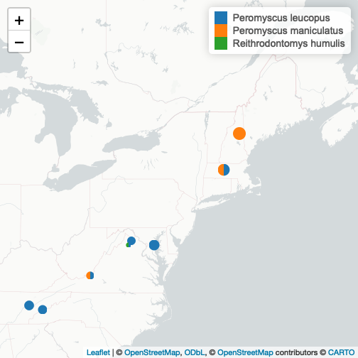 We see that we have a good representation of P. leucopus across our study area. For a strong species-specific analysis we may choose to focus on this species and investigate the CN ratios present at sites where it is present.
PleucSites <- mapSummaryWithSpecies[!is.na(mapSummaryWithSpecies$`Peromyscus leucopus`), ]


ggplot(PleucSites, aes(x = meanCN.ltr, y = meanCN.cfc)) +
  geom_point() +
  labs(
    x = "Litter CN ratio",
    y = "Canopy Foliage CN ratio",
  ) +
  theme_minimal()
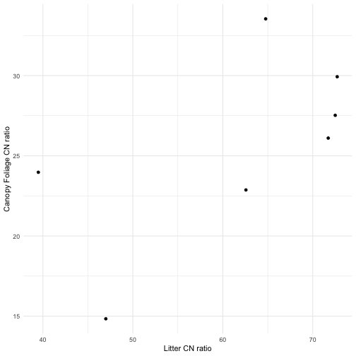
We see approximately 2-fold variation in both litter and canopy foliage CN ratios across these sites, indicating that a wide range of isotopic environments can be studied.
This is just one of many ways to connect NEON data with available organismal and environmental samples in order to develop new research projects. The Sample Portal allows you to search the fast growing collection of samples based on a variety of criteria, such as taxonomy, collecting events, preservation type, and more. You are encouraged to reach out via the NEON Biorepository Contact Form with any inquiries about NEON samples.