Tutorial
Merging AOP L3 Tiles in R into Full-Site Rasters
Last Updated: Apr 2, 2026
Most AOP L3 data are provided in 1km x 1km tiled geotiff rasters. A single site may contain hundreds of separate raster data files for each data product. This tutorial shows you how to merge these tiles into a single raster, covering the full site, which enables more efficient regional-scale analysis.
In this tutorial, you will import the aop_mosaic_rasters.R script and use the function
makeFullSiteMosaics to download AOP L3 tiled raster (geotiff) data sets for a
given data product, site, and year. This function uses the neonUtilities R package
byFileAOP function to download the data. Once downloaded, the tiles are merged
into a single raster covering the full site (or whatever coverage was obtained that year).
Finally, this full-site raster is saved as a geotiff and cloud-optimized geotiff
(COG) file in an output folder specified in the function.
Once you have generated full-site geotiffs, it is much simpler to visualize and conduct further analysis of the data in your preferred geospatial application, eg. ArcGIS, QGIS, or Google Earth Engine.
Learning Objectives
After completing this activity, you will be able to:
- Run the
makeFullSiteMosaicsfunction to:- download and merge AOP L3 geotiff rasters
- export the full site rasters to geotiffs and cloud-optimized geotiffs (COG)
- Read in and plot the full site geotiffs
Things You’ll Need To Complete This Tutorial
To complete this tutorial you will need
- The most current version of R and, preferably, RStudio installed on your computer.
- A NEON API token (optional, but recommended). If you haven't set up an API token, or used it in an R environment, please refer to the tutorial: NEON API Tokens in R
- You will need to install the following R packages, if they are not already installed:
R Libraries to Install:
-
neonUtilities:
install.packages('neonUtilities') -
terra:
install.packages('terra') -
data.table:
install.packages('data.table') -
docstring:
install.packages('docstring')
Data to Download
You do not need to download any data prior to running this tutorial, as you will
download AOP data sets using neonUtilities as part of this lesson.
Set Working Directory: This lesson assumes that you have set your working directory to the folder where you have cloned the github repo, and/or where you have saved the aop_merge_raster_functions.R script (code can be downloaded at the bottom of this tutorial). You will need to modify the working directory path in this tutorial to match your local directory structure.
An overview of setting the working directory in R can be found here.
Recommended Skills
For this tutorial you should be familiar with AOP data, and raster geotiff data generally.
You should also be familiar with the neonUtilities R package for downloading NEON data.
If you have not used a NEON token for downloading data, we recommend you review the tutorial Using an API Token when Accessing NEON Data with neonUtilities.
AOP Raster Data
The function makeFullSiteMosaics is set up for downloading AOP L3 lidar and
spectrometer derived raster data products. The table below shows a full list of
these data products, including the sensor, data product ID (dpID), the
sub-directory structure where files are downloaded to (the neonUtilities
function preserves the original folder structure of the data as it is stored by
NEON on Google Cloud Storage), and the name of the files. neonUtilities prints
out the full path where data and metadata are downloaded, but the script
aop_mosaic_rasters.R used in this tutorial goes a step further, and
automatically finds the path where data is downloaded, and handles some
additional data management (such as unzipping zipped folders) in order to
simplify pre-processing.
Refer to this table when using the function. If you select a dpID that is not in this list, the function will error out and display a table with the valid dpIDs, (similar to the table).
| Sensor | Data Product ID | Download Path | Short Name |
|---|---|---|---|
| Lidar | DP3.30024.001 | L3/DiscreteLidar/DTMGtif | DTM |
| Lidar | DP3.30024.001 | L3/DiscreteLidar/DSMGtif | DSM |
| Lidar | DP3.30015.001 | L3/DiscreteLidar/CanopyHeightModelGtif | CHM |
| Lidar | DP3.30025.001 | L3/DiscreteLidar/SlopeGtif | slope |
| Lidar | DP3.30025.001 | L3/DiscreteLidar/AspectGtif | aspect |
| Spectrometer | DP3.30011.001 | L3/Spectrometer/Albedo | albedo |
| Spectrometer | DP3.30012.001 | L3/Spectrometer/LAI | LAI |
| Spectrometer | DP3.30014.001 | L3/Spectrometer/FPAR | fPAR |
| Spectrometer | DP3.30019.001 | L3/Spectrometer/WaterIndices | WaterIndices |
| Spectrometer | DP3.30026.001 | L3/Spectrometer/VegIndices | VegetationIndices |
This tutorial illustrates the function for the NEON aquatic site MCRA (McRae Creek) in Domain 16, the Pacific Northwest. This site was chosen for demonstration because it is one of the smallest AOP sites, and therefore is quicker to download. Let's get started!
First, clone the git repository locally and set the working directory to where you cloned the data skills repository. You will need to modify the file path below to reflect where you have cloned the repository, or saved the aop_merge_raster_functions.R script.
# change the wd depending on your local environment

wd <- file.path(path.expand("~"),"GitHubRepos","NEON-Data-Skills","tutorials","R","AOP","AOP-L3-rasters")

setwd(wd)
First let's use source to pull in the aop_merge_raster_functions.R script, which is located in the working directory. For more details on what source does, please refer to the CU Earth Lab Tutorial on Source Functions in R
source("aop_merge_raster_functions.R")
Let's take a look at the input parameters for the function makeFullSiteMosaics. If you start to type this function in R, it should show you the required (and optional inputs). Below is some more detailed information about this function:
Description
This function 1) Runs the neonUtilities byFileAOP function to download NEON AOP data by site, year, and product (see byFileAOP documentation for additional details). 2) mosaics the data product tiles into a full-site mosaic, as well as the associated error tifs, where applicable, and 3) saves the full site mosaics to a tif and optional cloud-optimized geotiff.
Usage
makeFullSiteMosaics( dpID, year, siteCode, dataRootDir, outFileDir, include.provisional = T, apiToken = NULL, COG = T)
Arguments
dpID
The identifier of the AOP data product to download, in the form DP3.PRNUM.REV, e.g. DP3.30011.001. This works for all AOP L3 rasters except L3 reflectance. If an invalid data product ID is provided, the code will show an error message and display the valid dpIDs.
year
The four-digit year to search for data.
siteCode
The four-letter code of a single NEON site, e.g. 'MCRA'.
dataRootDir
The file path to download data to.
outFileDir
The file path where the full-site mosaic geotiffs and cloud-optimized geotiffs are saved.
include.provisional
T or F, should provisional data be included in downloaded files? Defaults to F. See https://www.neonscience.org/data-samples/data-management/data-revisions-releases for details on the difference between provisional and released data.
apiToken
User specific API token (generated within neon.datascience user accounts). If not provided, no API token is used.
COG
T or F, generate a Cloud Optimized Geotiff (COG) in addition to a geotiff? Defaults to F.
Data Tip: We recommend using an API token when downloading NEON data programmatically. The function will work without a token, if you leave it out (as described in the documentation), but it is best to get in the practice of using the token! Here I source the token from a file, where the file consists of a single line of code defining the token (called NEON_TOKEN). To set up an API token, please refer to the R tutorial on generating tokens, linked in the Recommended SKills section at the beginning of this lesson.
You can set the token as follows, directly in R, replacing "MY TOKEN" with your unique token.
NEON_TOKEN <- "MY TOKEN"
You can read in the token that is saved as neon_token.R using the source function as follows. This assumes the token is saved in the working directory, but you can also set the path to the token explicitly if you've saved it elsewhere.
source(paste0(wd,"/neon_token.R"))
Now that we have a general idea of how this function works, and have set the API TOKEN, let's go ahead and run the function.
For this example, the download folder is set to 'c:/neon/data' and the output folder to 'c:/neon/outputs/2021_MCRA/CHM/'. Modify these paths as desired according to your project structure.
Please heed the following warnings before you run the code:
WARNING: This function is currently set so that it does not check the file size before downloading. You can change this, if desired, by either removing the check.size parameter in the the makeFullSiteMosaics function, or by changing the value for that setting to True (check.size=T). This will pause the function and prompt you to type y/n (yes or no) to continue with the download. We recommend changing this parameter if you have limited storage space on your computer, but note that doing so will require a manual input to complete the execution of the function.
WARNING: We recommend extending the timeout value when downloading large AOP sites so the connection doesn't stall out before the files finished downloading. To change this setting, you can the R options, but note that this will change the computer's settings outside of this R environment. If you do re-set the timeout, be sure to change it back at the end. The default timeout is 60 seconds, we recommend changing it to 300 seconds (5 minutes).
timeout0 <- getOption('timeout')

print(timeout0)

## [1] 60
Set the timeout to 300 seconds (5 minutes):
options(timeout=300)

getOption('timeout')

## [1] 300
Set the folder to download the data to, and the output folder to save the final CHM rasters:
download_folder <- 'c:/neon/data'

chm_output_folder <- 'c:/neon/outputs/2021_MCRA/CHM/'
Now we're ready to run the makeFullSiteMosaics function. We will set include.provisional=T to include provisional data (by default it is set to False). That shouldn't matter in this case because the 2021 MCRA data is part of a Release. For more information on provisional v. released data, please refer to the tutorial:
Understanding Releases and Provisional Data
makeFullSiteMosaics('DP3.30015.001','2021','MCRA',download_folder,chm_output_folder,NEON_TOKEN,include.provisional=T,COG=T)
Display the output files generated:
list.files(chm_output_folder)

## [1] "2021_MCRA_2_CHM.tif"     "2021_MCRA_2_CHM_COG.tif" "2022_MCRA_3_CHM.tif"     "2022_MCRA_3_CHM_COG.tif"
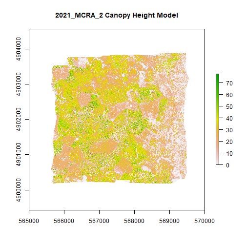
Now we can read in and plot the full-site CHM tif that we generated using the raster package:
MCRA_CHM <- rast(file.path(chm_output_folder,'2021_MCRA_2_CHM.tif'))

plot(MCRA_CHM,main="2021_MCRA_2 Canopy Height Model") # add title with main)
Now let's run the function to generate full-site mosaics for the AOP Veg Indices (DP3.30026.001). The function handles unzipping the zipped folders, and plotting each separate index tif and associated error tif. We will use the same download folder as before (note that the files will be downloaded to a different sub-directory), and specify a new output folder.
Now we will run makeFullSiteMosaics again. This time leave out the include.provisional parameter, since it is set to False by default. This time we'll leave the defaults for include.provisional and COG, so COGs will not be generated.
veg_indices_output_folder<-'c:/neon/outputs/2021_MCRA/VegIndices/'

makeFullSiteMosaics('DP3.30026.001','2021','MCRA',download_folder,veg_indices_output_folder,NEON_TOKEN)
Let's see the full-site Veg Indices files that were generated using list.files:
list.files(veg_indices_output_folder)

##  [1] "2021_MCRA_2_ARVI.tif"       "2021_MCRA_2_ARVI_error.tif" "2021_MCRA_2_EVI.tif"        "2021_MCRA_2_EVI_error.tif"
##  [5] "2021_MCRA_2_NDVI.tif"       "2021_MCRA_2_NDVI_error.tif" "2021_MCRA_2_PRI.tif"        "2021_MCRA_2_PRI_error.tif"
##  [9] "2021_MCRA_2_SAVI.tif"       "2021_MCRA_2_SAVI_error.tif"
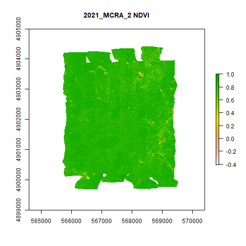
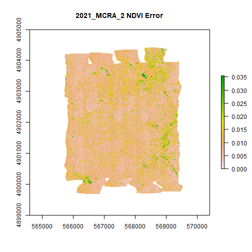
Now we can read in the NDVI and NDVI error tifs:
MCRA_NDVI <- rast(file.path(veg_indices_output_folder,'2021_MCRA_2_NDVI.tif'))

MCRA_NDVI_error <- rast(file.path(veg_indices_output_folder,'2021_MCRA_2_NDVI_error.tif'))
And, finally, let's plot NDVI and NDVI error:
plot(MCRA_NDVI,main="2021_MCRA_2 NDVI")
plot(MCRA_NDVI_error,main="2021_MCRA_2 NDVI Error")
 Looks good! Go ahead and test out this function on different data products, years, or sites on your own. Note that larger sites will take more time to download the data, and may require significant memory resources on your computer.
Last but not least, change the timeout back to the original value:
options(timeout=timeout0)

getOption('timeout')

## [1] 60