Tutorial

Vector 01: Explore Shapefile Attributes & Plot Shapefile Objects by Attribute Value in R

Authors: Joseph Stachelek, Leah A. Wasser, Megan A. Jones

Last Updated: Apr 8, 2021

This tutorial explains what shapefile attributes are and how to work with shapefile attributes in R. It also covers how to identify and query shapefile attributes, as well as subset shapefiles by specific attribute values. Finally, we will review how to plot a shapefile according to a set of attribute values.

Learning Objectives

After completing this tutorial, you will be able to:

Query shapefile attributes.
Subset shapefiles using specific attribute values.
Plot a shapefile, colored by unique attribute values.

Things You’ll Need To Complete This Tutorial

You will need the most current version of R and, preferably, RStudio loaded on your computer to complete this tutorial.

Install R Packages

raster: install.packages("raster")
rgdal: install.packages("rgdal")
sp: install.packages("sp")

More on Packages in R – Adapted from Software Carpentry.

Download Data

NEON Teaching Data Subset: Site Layout Shapefiles

These vector data provide information on the site characterization and infrastructure at the National Ecological Observatory Network's Harvard Forest field site. The Harvard Forest shapefiles are from the Harvard Forest GIS & Map archives. US Country and State Boundary layers are from the US Census Bureau.

Download Dataset

Set Working Directory: This lesson assumes that you have set your working directory to the location of the downloaded and unzipped data subsets.

An overview of setting the working directory in R can be found here.

R Script & Challenge Code: NEON data lessons often contain challenges that reinforce learned skills. If available, the code for challenge solutions is found in the downloadable R script of the entire lesson, available in the footer of each lesson page.

Shapefile Metadata & Attributes

When we import a shapefile into R, the readOGR() function automatically stores metadata and attributes associated with the file.

Load the Data

To work with vector data in R, we can use the rgdal library. The raster package also allows us to explore metadata using similar commands for both raster and vector files.

We will import three shapefiles. The first is our AOI or area of interest boundary polygon that we worked with in Open and Plot Shapefiles in R. The second is a shapefile containing the location of roads and trails within the field site. The third is a file containing the Fisher tower location.

If you completed the Open and Plot Shapefiles in R. tutorial, you can skip this code.

# load packages
# rgdal: for vector work; sp package should always load with rgdal. 
library(rgdal)  
# raster: for metadata/attributes- vectors or rasters
library (raster)   

# set working directory to data folder
# setwd("pathToDirHere")

# Import a polygon shapefile
aoiBoundary_HARV <- readOGR("NEON-DS-Site-Layout-Files/HARV",
                            "HarClip_UTMZ18", stringsAsFactors = T)

## OGR data source with driver: ESRI Shapefile 
## Source: "/Users/olearyd/Git/data/NEON-DS-Site-Layout-Files/HARV", layer: "HarClip_UTMZ18"
## with 1 features
## It has 1 fields
## Integer64 fields read as strings:  id

# Import a line shapefile
lines_HARV <- readOGR( "NEON-DS-Site-Layout-Files/HARV", "HARV_roads", stringsAsFactors = T)

## OGR data source with driver: ESRI Shapefile 
## Source: "/Users/olearyd/Git/data/NEON-DS-Site-Layout-Files/HARV", layer: "HARV_roads"
## with 13 features
## It has 15 fields

# Import a point shapefile 
point_HARV <- readOGR("NEON-DS-Site-Layout-Files/HARV",
                      "HARVtower_UTM18N", stringsAsFactors = T)

## OGR data source with driver: ESRI Shapefile 
## Source: "/Users/olearyd/Git/data/NEON-DS-Site-Layout-Files/HARV", layer: "HARVtower_UTM18N"
## with 1 features
## It has 14 fields

Query Shapefile Metadata

Remember, as covered in Open and Plot Shapefiles in R., we can view metadata associated with an R object using:

class() - Describes the type of vector data stored in the object.
length() - How many features are in this spatial object?
object extent() - The spatial extent (geographic area covered by) features in the object.
coordinate reference system (crs()) - The spatial projection that the data are in.

Let's explore the metadata for our point_HARV object.

# view class
class(x = point_HARV)

## [1] "SpatialPointsDataFrame"
## attr(,"package")
## [1] "sp"

# x= isn't actually needed; it just specifies which object
# view features count
length(point_HARV)

## [1] 1

# view crs - note - this only works with the raster package loaded
crs(point_HARV)

## CRS arguments:
##  +proj=utm +zone=18 +datum=WGS84 +units=m +no_defs

# view extent- note - this only works with the raster package loaded
extent(point_HARV)

## class      : Extent 
## xmin       : 732183.2 
## xmax       : 732183.2 
## ymin       : 4713265 
## ymax       : 4713265

# view metadata summary
point_HARV

## class       : SpatialPointsDataFrame 
## features    : 1 
## extent      : 732183.2, 732183.2, 4713265, 4713265  (xmin, xmax, ymin, ymax)
## crs         : +proj=utm +zone=18 +datum=WGS84 +units=m +no_defs 
## variables   : 14
## names       : Un_ID, Domain, DomainName,       SiteName, Type,       Sub_Type,     Lat,      Long, Zone,       Easting,       Northing,                Ownership,    County, annotation 
## value       :     A,      1,  Northeast, Harvard Forest, Core, Advanced Tower, 42.5369, -72.17266,   18, 732183.193774, 4713265.041137, Harvard University, LTER, Worcester,         C1

About Shapefile Attributes

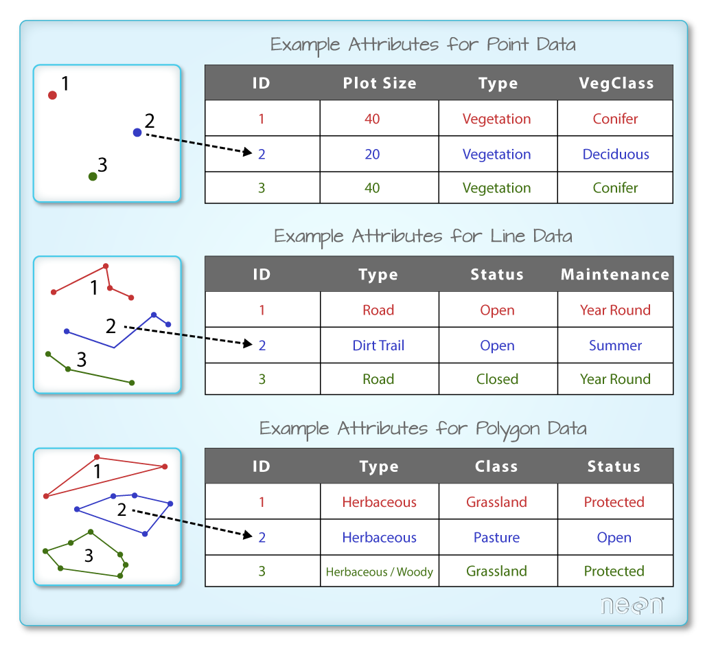
Shapefiles often contain an associated database or spreadsheet of values called attributes that describe the vector features in the shapefile. You can think of this like a spreadsheet with rows and columns. Each column in the spreadsheet is an individual attribute that describes an object. Shapefile attributes include measurements that correspond to the geometry of the shapefile features.

For example, the HARV_Roads shapefile (lines_HARV object) contains an attribute called TYPE. Each line in the shapefile has an associated TYPE which describes the type of road (woods road, footpath, boardwalk, or stone wall).

Example attribute tables for each different type of vector object. — The shapefile format allows us to store attributes for each feature (vector object) stored in the shapefile. The attribute table is similar to a spreadsheet. There is a row for each feature. The first column contains the unique ID of the feature. We can add additional columns that describe the feature. Image Source: National Ecological Observatory Network (NEON)

We can look at all of the associated data attributes by printing the contents of the data slot with objectName@data. We can use the base R length function to count the number of attributes associated with a spatial object too.

# just view the attributes & first 6 attribute values of the data
head(lines_HARV@data)

##   OBJECTID_1 OBJECTID       TYPE             NOTES MISCNOTES RULEID
## 0         14       48 woods road Locust Opening Rd      <NA>      5
## 1         40       91   footpath              <NA>      <NA>      6
## 2         41      106   footpath              <NA>      <NA>      6
## 3        211      279 stone wall              <NA>      <NA>      1
## 4        212      280 stone wall              <NA>      <NA>      1
## 5        213      281 stone wall              <NA>      <NA>      1
##            MAPLABEL SHAPE_LENG             LABEL BIKEHORSE RESVEHICLE
## 0 Locust Opening Rd 1297.35706 Locust Opening Rd         Y         R1
## 1              <NA>  146.29984              <NA>         Y         R1
## 2              <NA>  676.71804              <NA>         Y         R2
## 3              <NA>  231.78957              <NA>      <NA>       <NA>
## 4              <NA>   45.50864              <NA>      <NA>       <NA>
## 5              <NA>  198.39043              <NA>      <NA>       <NA>
##   RECMAP Shape_Le_1                            ResVehic_1
## 0      Y 1297.10617    R1 - All Research Vehicles Allowed
## 1      Y  146.29983    R1 - All Research Vehicles Allowed
## 2      Y  676.71807 R2 - 4WD/High Clearance Vehicles Only
## 3   <NA>  231.78962                                  <NA>
## 4   <NA>   45.50859                                  <NA>
## 5   <NA>  198.39041                                  <NA>
##                    BicyclesHo
## 0 Bicycles and Horses Allowed
## 1 Bicycles and Horses Allowed
## 2 Bicycles and Horses Allowed
## 3                        <NA>
## 4                        <NA>
## 5                        <NA>

# how many attributes are in our vector data object?
length(lines_HARV@data)

## [1] 15

We can view the individual name of each attribute using the names(lines_HARV@data) method in R. We could also view just the first 6 rows of attribute values using head(lines_HARV@data).

Let's give it a try.

# view just the attribute names for the lines_HARV spatial object
names(lines_HARV@data)

##  [1] "OBJECTID_1" "OBJECTID"   "TYPE"       "NOTES"      "MISCNOTES" 
##  [6] "RULEID"     "MAPLABEL"   "SHAPE_LENG" "LABEL"      "BIKEHORSE" 
## [11] "RESVEHICLE" "RECMAP"     "Shape_Le_1" "ResVehic_1" "BicyclesHo"

### Challenge: Attributes for Different Spatial Classes Explore the attributes associated with the `point_HARV` and `aoiBoundary_HARV` spatial objects.

How many attributes do each have?
Who owns the site in the point_HARV data object?
Which of the following is NOT an attribute of the point data object?

A) Latitude B) County C) Country

Explore Values within One Attribute

We can explore individual values stored within a particular attribute. Again, comparing attributes to a spreadsheet or a data.frame is similar to exploring values in a column. We can do this using the $ and the name of the attribute: objectName$attributeName.

# view all attributes in the lines shapefile within the TYPE field
lines_HARV$TYPE

##  [1] woods road footpath   footpath   stone wall stone wall stone wall
##  [7] stone wall stone wall stone wall boardwalk  woods road woods road
## [13] woods road
## Levels: boardwalk footpath stone wall woods road

# view unique values within the "TYPE" attributes
levels(lines_HARV@data$TYPE)

## [1] "boardwalk"  "footpath"   "stone wall" "woods road"

Notice that two of our TYPE attribute values consist of two separate words: stone wall and woods road. There are really four unique TYPE values, not six TYPE values.

Subset Shapefiles

We can use the objectName$attributeName syntax to select a subset of features from a spatial object in R.

# select features that are of TYPE "footpath"
# could put this code into other function to only have that function work on
# "footpath" lines
lines_HARV[lines_HARV$TYPE == "footpath",]

## class       : SpatialLinesDataFrame 
## features    : 2 
## extent      : 731954.5, 732232.3, 4713131, 4713726  (xmin, xmax, ymin, ymax)
## crs         : +proj=utm +zone=18 +datum=WGS84 +units=m +no_defs 
## variables   : 15
## names       : OBJECTID_1, OBJECTID,     TYPE, NOTES, MISCNOTES, RULEID, MAPLABEL,    SHAPE_LENG, LABEL, BIKEHORSE, RESVEHICLE, RECMAP,    Shape_Le_1,                            ResVehic_1,                  BicyclesHo 
## min values  :         40,       91, footpath,    NA,        NA,      6,       NA, 146.299844868,    NA,         Y,         R1,      Y, 146.299831389,    R1 - All Research Vehicles Allowed, Bicycles and Horses Allowed 
## max values  :         41,      106, footpath,    NA,        NA,      6,       NA,  676.71804248,    NA,         Y,         R2,      Y, 676.718065323, R2 - 4WD/High Clearance Vehicles Only, Bicycles and Horses Allowed

# save an object with only footpath lines
footpath_HARV <- lines_HARV[lines_HARV$TYPE == "footpath",]
footpath_HARV

## class       : SpatialLinesDataFrame 
## features    : 2 
## extent      : 731954.5, 732232.3, 4713131, 4713726  (xmin, xmax, ymin, ymax)
## crs         : +proj=utm +zone=18 +datum=WGS84 +units=m +no_defs 
## variables   : 15
## names       : OBJECTID_1, OBJECTID,     TYPE, NOTES, MISCNOTES, RULEID, MAPLABEL,    SHAPE_LENG, LABEL, BIKEHORSE, RESVEHICLE, RECMAP,    Shape_Le_1,                            ResVehic_1,                  BicyclesHo 
## min values  :         40,       91, footpath,    NA,        NA,      6,       NA, 146.299844868,    NA,         Y,         R1,      Y, 146.299831389,    R1 - All Research Vehicles Allowed, Bicycles and Horses Allowed 
## max values  :         41,      106, footpath,    NA,        NA,      6,       NA,  676.71804248,    NA,         Y,         R2,      Y, 676.718065323, R2 - 4WD/High Clearance Vehicles Only, Bicycles and Horses Allowed

# how many features are in our new object
length(footpath_HARV)

## [1] 2

Our subsetting operation reduces the features count from 13 to 2. This means that only two feature lines in our spatial object have the attribute "TYPE=footpath".

We can plot our subsetted shapefiles.

# plot just footpaths
plot(footpath_HARV,
     lwd=6,
     main="NEON Harvard Forest Field Site\n Footpaths")

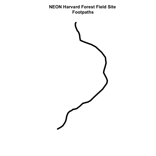
Foothpaths at NEON Harvard Forest Field Site.

Interesting! Above, it appeared as if we had 2 features in our footpaths subset. Why does the plot look like there is only one feature?

Let's adjust the colors used in our plot. If we have 2 features in our vector object, we can plot each using a unique color by assigning unique colors (col=) to our features. We use the syntax

col="c("colorOne","colorTwo")

to do this.

# plot just footpaths
plot(footpath_HARV,
     col=c("green","blue"), # set color for each feature 
     lwd=6,
     main="NEON Harvard Forest Field Site\n Footpaths \n Feature one = blue, Feature two= green")

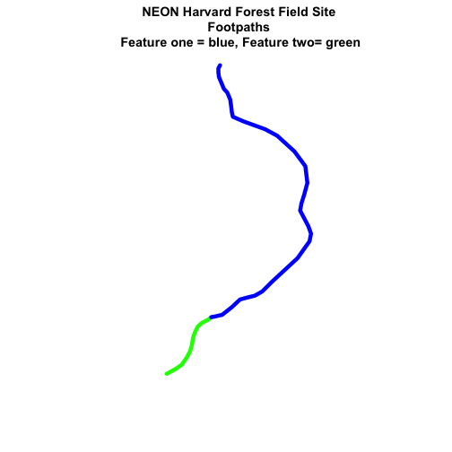
Foothpaths at NEON Harvard Forest Field Site with color varied by feature type.

Now, we see that there are in fact two features in our plot!

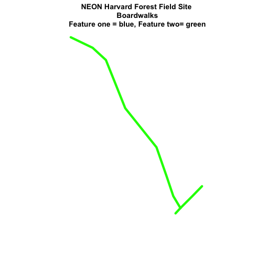
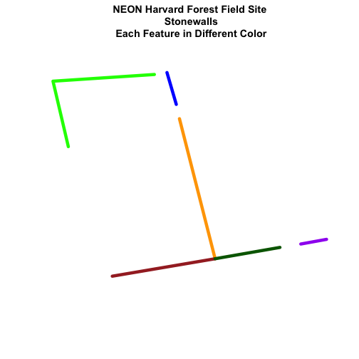
### Challenge: Subset Spatial Line Objects Subset out all:

boardwalk from the lines layer and plot it.
stone wall features from the lines layer and plot it.

For each plot, color each feature using a unique color.

Boardwalks at NEON Harvard Forest Field Site with color varied by feature type. Stone walls at NEON Harvard Forest Field Site with color varied by feature type.

Plot Lines by Attribute Value

To plot vector data with the color determined by a set of attribute values, the attribute values must be class = factor. A factor is similar to a category.

you can group vector objects by a particular category value - for example you can group all lines of TYPE=footpath. However, in R, a factor can also have a determined order.

By default, R will import spatial object attributes as factors.

**Data Tip:** If our data attribute values are not read in as factors, we can convert the categorical attribute values using `as.factor()`.

# view the original class of the TYPE column
class(lines_HARV$TYPE)

## [1] "factor"

# view levels or categories - note that there are no categories yet in our data!
# the attributes are just read as a list of character elements.
levels(lines_HARV$TYPE)

## [1] "boardwalk"  "footpath"   "stone wall" "woods road"

# Convert the TYPE attribute into a factor
# Only do this IF the data do not import as a factor!
# lines_HARV$TYPE <- as.factor(lines_HARV$TYPE)
# class(lines_HARV$TYPE)
# levels(lines_HARV$TYPE)

# how many features are in each category or level?
summary(lines_HARV$TYPE)

##  boardwalk   footpath stone wall woods road 
##          1          2          6          4

When we use plot(), we can specify the colors to use for each attribute using the col= element. To ensure that R renders each feature by it's associated factor / attribute value, we need to create a vector or colors - one for each feature, according to it's associated attribute value / factor value.

To create this vector we can use the following syntax:

c("colorOne", "colorTwo","colorThree")[object$factor]

Note in the above example we have:

a vector of colors - one for each factor value (unique attribute value)
the attribute itself ([object$factor]) of class factor

Let's give this a try.

# Check the class of the attribute - is it a factor?
class(lines_HARV$TYPE)

## [1] "factor"

# how many "levels" or unique values does the factor have?
# view factor values
levels(lines_HARV$TYPE)

## [1] "boardwalk"  "footpath"   "stone wall" "woods road"

# count the number of unique values or levels
length(levels(lines_HARV$TYPE))

## [1] 4

# create a color palette of 4 colors - one for each factor level
roadPalette <- c("blue","green","grey","purple")
roadPalette

## [1] "blue"   "green"  "grey"   "purple"

# create a vector of colors - one for each feature in our vector object
# according to its attribute value
roadColors <- c("blue","green","grey","purple")[lines_HARV$TYPE]
roadColors

##  [1] "purple" "green"  "green"  "grey"   "grey"   "grey"   "grey"  
##  [8] "grey"   "grey"   "blue"   "purple" "purple" "purple"

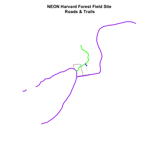
# plot the lines data, apply a diff color to each factor level)
plot(lines_HARV, 
     col=roadColors,
     lwd=3,
     main="NEON Harvard Forest Field Site\n Roads & Trails")

Roads and trails at NEON Harvard Forest Field Site with color varied by attribute factor level.

Adjust Line Width

We can also adjust the width of our plot lines using lwd. We can set all lines to be thicker or thinner using lwd=.

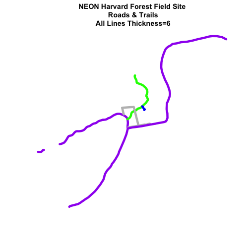
# make all lines thicker
plot(lines_HARV, 
     col=roadColors,
     main="NEON Harvard Forest Field Site\n Roads & Trails\n All Lines Thickness=6",
     lwd=6)

Roads and trails at NEON Harvard Forest Field Site with color varied by attribute factor value and uniformly thick line width.

Adjust Line Width by Attribute

If we want a unique line width for each factor level or attribute category in our spatial object, we can use the same syntax that we used for colors, above:

lwd=c("widthOne", "widthTwo","widthThree")[object$factor]

Note that this requires the attribute to be of class factor. Let's give it a try.

class(lines_HARV$TYPE)

## [1] "factor"

levels(lines_HARV$TYPE)

## [1] "boardwalk"  "footpath"   "stone wall" "woods road"

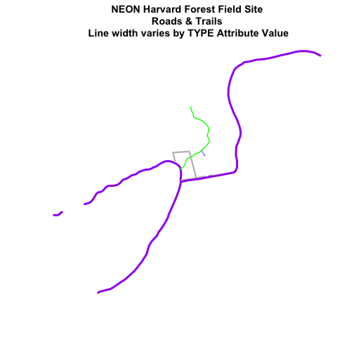
# create vector of line widths
lineWidths <- (c(1,2,3,4))[lines_HARV$TYPE]
# adjust line width by level
# in this case, boardwalk (the first level) is the widest.
plot(lines_HARV, 
     col=roadColors,
     main="NEON Harvard Forest Field Site\n Roads & Trails \n Line width varies by TYPE Attribute Value",
     lwd=lineWidths)

Roads and trails at NEON Harvard Forest Field Site with color and line width varied by attribute factor value.

### Challenge: Plot Line Width by Attribute We can customize the width of each line, according to specific attribute value, too. To do this, we create a vector of line width values, and map that vector to the factor levels - using the same syntax that we used above for colors. HINT: `lwd=(vector of line width thicknesses)[spatialObject$factorAttribute]`

Create a plot of roads using the following line thicknesses:

woods road lwd=8
Boardwalks lwd = 2
footpath lwd=4
stone wall lwd=3

Roads and trails at NEON Harvard Forest Field Site with color and line width varied by specific attribute value.

**Data Tip:** Given we have a factor with 4 levels, we can create an vector of numbers, each of which specifies the thickness of each feature in our `SpatialLinesDataFrame` by factor level (category): `c(6,4,1,2)[lines_HARV$TYPE]`

Add Plot Legend

We can add a legend to our plot too. When we add a legend, we use the following elements to specify labels and colors:

bottomright: We specify the location of our legend by using a default keyword. We could also use top, topright, etc.
levels(objectName$attributeName): Label the legend elements using the categories of levels in an attribute (e.g., levels(lines_HARV$TYPE) means use the levels boardwalk, footpath, etc).
fill=: apply unique colors to the boxes in our legend. palette() is the default set of colors that R applies to all plots.

Let's add a legend to our plot.

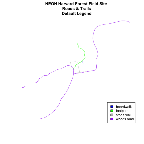
plot(lines_HARV, 
     col=roadColors,
     main="NEON Harvard Forest Field Site\n Roads & Trails\n Default Legend")

# we can use the color object that we created above to color the legend objects
roadPalette

## [1] "blue"   "green"  "grey"   "purple"

# add a legend to our map
legend("bottomright",   # location of legend
      legend=levels(lines_HARV$TYPE), # categories or elements to render in 
			 # the legend
      fill=roadPalette) # color palette to use to fill objects in legend.

Roads and trails at NEON Harvard Forest Field Site with color varied by attribute factor value and with a default legend.

We can tweak the appearance of our legend too.

bty=n: turn off the legend BORDER
cex: change the font size

Let's try it out.

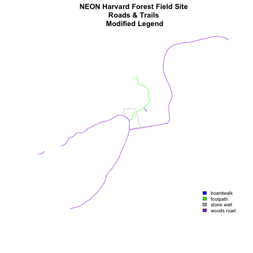
plot(lines_HARV, 
     col=roadColors,
     main="NEON Harvard Forest Field Site\n Roads & Trails \n Modified Legend")
# add a legend to our map
legend("bottomright", 
       legend=levels(lines_HARV$TYPE), 
       fill=roadPalette, 
       bty="n", # turn off the legend border
       cex=.8) # decrease the font / legend size

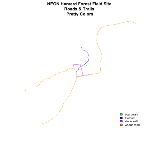
Roads and trails at NEON Harvard Forest Field Site with color varied by attribute factor value and with a modified legend.

We can modify the colors used to plot our lines by creating a new color vector directly in the plot code rather than creating a separate object.

col=(newColors)[lines_HARV$TYPE]

Let's try it!

# manually set the colors for the plot!
newColors <- c("springgreen", "blue", "magenta", "orange")
newColors

## [1] "springgreen" "blue"        "magenta"     "orange"

# plot using new colors
plot(lines_HARV, 
     col=(newColors)[lines_HARV$TYPE],
     main="NEON Harvard Forest Field Site\n Roads & Trails \n Pretty Colors")

# add a legend to our map
legend("bottomright", 
       levels(lines_HARV$TYPE), 
       fill=newColors, 
       bty="n", cex=.8)

Roads and trails at NEON Harvard Forest Field Site with manually set colors and with a modified legend.

**Data Tip:** You can modify the default R color palette using the palette method. For example `palette(rainbow(6))` or `palette(terrain.colors(6))`. You can reset the palette colors using `palette("default")`!

### Challenge: Plot Lines by Attribute Create a plot that emphasizes only roads where bicycles and horses are allowed. To emphasize this, make the lines where bicycles are not allowed THINNER than the roads where bicycles are allowed. NOTE: this attribute information is located in the `lines_HARV$BicyclesHo` attribute.

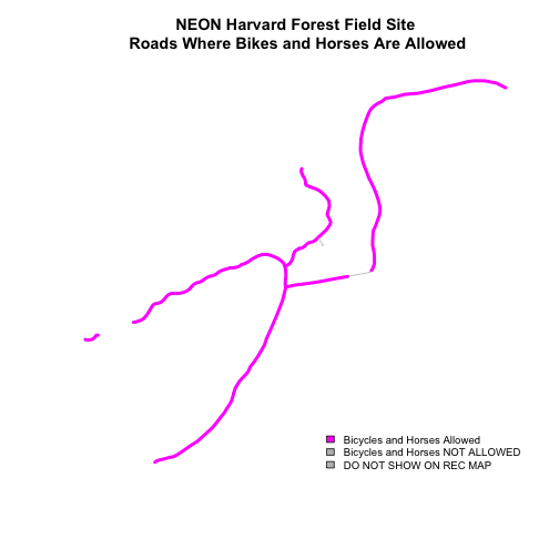
Be sure to add a title and legend to your map! You might consider a color palette that has all bike/horse-friendly roads displayed in a bright color. All other lines can be grey.

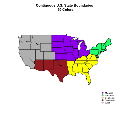
Roads where Bikes and Horses are Allowed on NEON Harvard Forest Field Site with lines varied by attribute factor and with a modified legend.

### Challenge: Plot Polygon by Attribute

Create a map of the State boundaries in the United States using the data located in your downloaded data folder: NEON-DS-Site-Layout-Files/US-Boundary-Layers\US-State-Boundaries-Census-2014. Apply a fill color to each state using its region value. Add a legend.
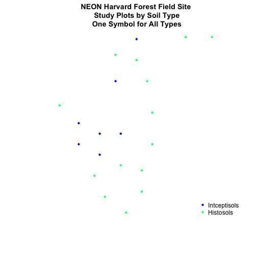
Using the NEON-DS-Site-Layout-Files/HARV/PlotLocations_HARV.shp shapefile, create a map of study plot locations, with each point colored by the soil type (soilTypeOr). Question: How many different soil types are there at this particular field site?
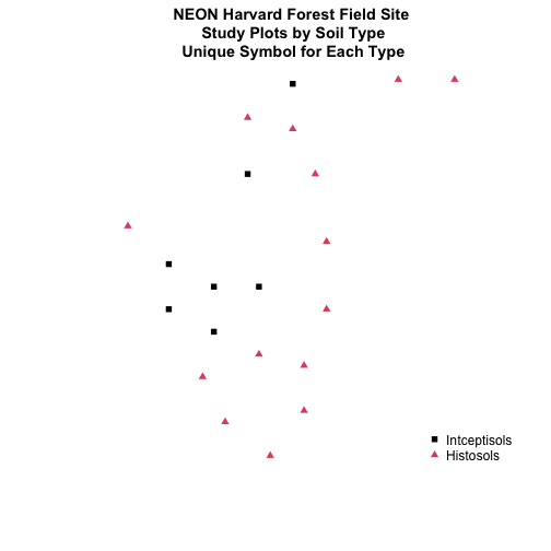
BONUS -- modify the field site plot above. Plot each point, using a different symbol. HINT: you can assign the symbol using pch= value. You can create a vector object of symbols by factor level using the syntax syntax that we used above to create a vector of lines widths and colors: pch=c(15,17)[lines_HARV$soilTypeOr]. Type ?pch to learn more about pch or use google to find a list of pch symbols that you can use in R.

Contiguous U.S. State Boundaries with color varied by region and with a modified legend. Soil Study Plots by Soil Type at NEON Harvard Forest Field Site with color varied by type and one symbol for all types and with a modified legend.