Vector 02: Plot Multiple Shapefiles and Create Custom Legends in Base Plot in R

This tutorial builds upon the previous tutorial, to work with shapefile attributes in R and explores how to plot multiple shapefiles using base R graphics. It then covers how to create a custom legend with colors and symbols that match your plot.

Load the Data

To work with vector data in R, we can use the rgdal library. The raster package also allows us to explore metadata using similar commands for both raster and vector files.

We will import three shapefiles. The first is our AOI or area of interest boundary polygon that we worked with in Open and Plot Shapefiles in R. The second is a shapefile containing the location of roads and trails within the field site. The third is a file containing the Harvard Forest Fisher tower location. These latter two we worked with in the Explore Shapefile Attributes & Plot Shapefile Objects by Attribute Value in R tutorial.

# load packages
# rgdal: for vector work; sp package should always load with rgdal. 
library(rgdal)  
# raster: for metadata/attributes- vectors or rasters
library(raster)   

# set working directory to data folder
# setwd("pathToDirHere")

# Import a polygon shapefile 
aoiBoundary_HARV <- readOGR("NEON-DS-Site-Layout-Files/HARV",
                            "HarClip_UTMZ18", stringsAsFactors = T)

## OGR data source with driver: ESRI Shapefile 
## Source: "/Users/olearyd/Git/data/NEON-DS-Site-Layout-Files/HARV", layer: "HarClip_UTMZ18"
## with 1 features
## It has 1 fields
## Integer64 fields read as strings:  id

# Import a line shapefile
lines_HARV <- readOGR( "NEON-DS-Site-Layout-Files/HARV", "HARV_roads", stringsAsFactors = T)

## OGR data source with driver: ESRI Shapefile 
## Source: "/Users/olearyd/Git/data/NEON-DS-Site-Layout-Files/HARV", layer: "HARV_roads"
## with 13 features
## It has 15 fields

# Import a point shapefile 
point_HARV <- readOGR("NEON-DS-Site-Layout-Files/HARV",
                      "HARVtower_UTM18N", stringsAsFactors = T)

## OGR data source with driver: ESRI Shapefile 
## Source: "/Users/olearyd/Git/data/NEON-DS-Site-Layout-Files/HARV", layer: "HARVtower_UTM18N"
## with 1 features
## It has 14 fields

Plot Data

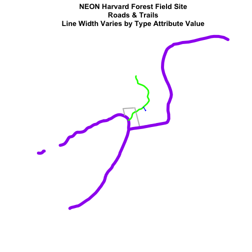
In the Explore Shapefile Attributes & Plot Shapefile Objects by Attribute Value in R tutorial we created a plot where we customized the width of each line in a spatial object according to a factor level or category. To do this, we create a vector of colors containing a color value for EACH feature in our spatial object grouped by factor level or category.

# view the factor levels
levels(lines_HARV$TYPE)

## [1] "boardwalk"  "footpath"   "stone wall" "woods road"

# create vector of line width values
lineWidth <- c(2,4,3,8)[lines_HARV$TYPE]
# view vector
lineWidth

##  [1] 8 4 4 3 3 3 3 3 3 2 8 8 8

# create a color palette of 4 colors - one for each factor level
roadPalette <- c("blue","green","grey","purple")
roadPalette

## [1] "blue"   "green"  "grey"   "purple"

# create a vector of colors - one for each feature in our vector object
# according to its attribute value
roadColors <- c("blue","green","grey","purple")[lines_HARV$TYPE]
roadColors

##  [1] "purple" "green"  "green"  "grey"   "grey"   "grey"   "grey"  
##  [8] "grey"   "grey"   "blue"   "purple" "purple" "purple"

# create vector of line width values
lineWidth <- c(2,4,3,8)[lines_HARV$TYPE]
# view vector
lineWidth

##  [1] 8 4 4 3 3 3 3 3 3 2 8 8 8

# in this case, boardwalk (the first level) is the widest.
plot(lines_HARV, 
     col=roadColors,
     main="NEON Harvard Forest Field Site\n Roads & Trails \nLine Width Varies by Type Attribute Value",
     lwd=lineWidth)

Add Plot Legend

In the the previous tutorial, we also learned how to add a basic legend to our plot.

• bottomright: We specify the location of our legend by using a default keyword. We could also use top, topright, etc.
• levels(objectName$attributeName): Label the legend elements using the categories of levels in an attribute (e.g., levels(lines_HARV$TYPE) means use the levels boardwalk, footpath, etc).
• fill=: apply unique colors to the boxes in our legend. palette() is the default set of colors that R applies to all plots.

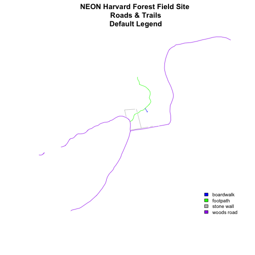
Let's add a legend to our plot.

plot(lines_HARV, 
     col=roadColors,
     main="NEON Harvard Forest Field Site\n Roads & Trails\n Default Legend")

# we can use the color object that we created above to color the legend objects
roadPalette

## [1] "blue"   "green"  "grey"   "purple"

# add a legend to our map
legend("bottomright", 
       legend=levels(lines_HARV$TYPE), 
       fill=roadPalette, 
       bty="n", # turn off the legend border
       cex=.8) # decrease the font / legend size

However, what if we want to create a more complex plot with many shapefiles and unique symbols that need to be represented clearly in a legend?

Plot Multiple Vector Layers

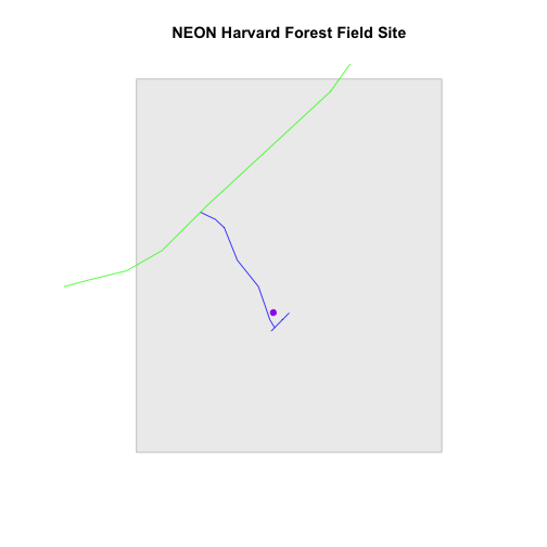
Now, let's create a plot that combines our tower location (point_HARV), site boundary (aoiBoundary_HARV) and roads (lines_HARV) spatial objects. We will need to build a custom legend as well.

To begin, create a plot with the site boundary as the first layer. Then layer the tower location and road data on top using add=TRUE.

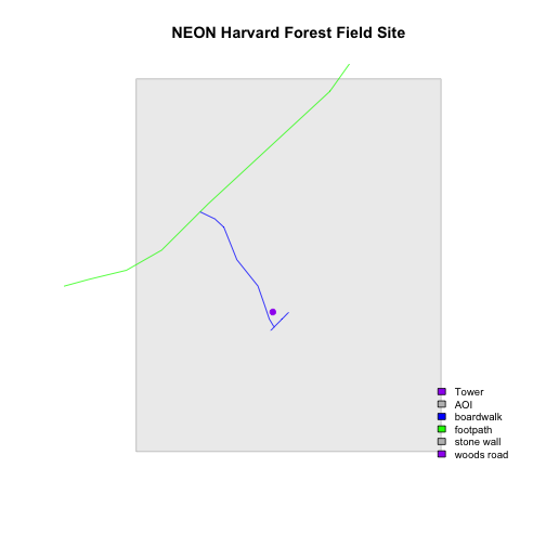
# Plot multiple shapefiles
plot(aoiBoundary_HARV, 
     col = "grey93", 
     border="grey",
     main="NEON Harvard Forest Field Site")

plot(lines_HARV, 
     col=roadColors,
     add = TRUE)

plot(point_HARV, 
     add  = TRUE, 
     pch = 19, 
     col = "purple")

# assign plot to an object for easy modification!
plot_HARV<- recordPlot()

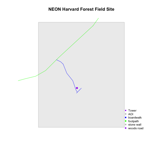
Customize Your Legend

Next, let's build a custom legend using the symbology (the colors and symbols) that we used to create the plot above. To do this, we will need to build three things:

1. A list of all "labels" (the text used to describe each element in the legend to use in the legend.
2. A list of colors used to color each feature in our plot.
3. A list of symbols to use in the plot. NOTE: we have a combination of points, lines and polygons in our plot. So we will need to customize our symbols!

Let's create objects for the labels, colors and symbols so we can easily reuse them. We will start with the labels.

# create a list of all labels
labels <- c("Tower", "AOI", levels(lines_HARV$TYPE))
labels

## [1] "Tower"      "AOI"        "boardwalk"  "footpath"   "stone wall"
## [6] "woods road"

# render plot
plot_HARV

# add a legend to our map
legend("bottomright", 
       legend=labels, 
       bty="n", # turn off the legend border
       cex=.8) # decrease the font / legend size

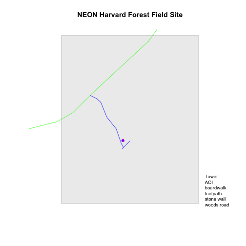
Now we have a legend with the labels identified. Let's add colors to each legend element next. We can use the vectors of colors that we created earlier to do this.

# we have a list of colors that we used above - we can use it in the legend
roadPalette

## [1] "blue"   "green"  "grey"   "purple"

# create a list of colors to use 
plotColors <- c("purple", "grey", roadPalette)
plotColors

## [1] "purple" "grey"   "blue"   "green"  "grey"   "purple"

# render plot
plot_HARV

# add a legend to our map
legend("bottomright", 
       legend=labels, 
       fill=plotColors,
       bty="n", # turn off the legend border
       cex=.8) # decrease the font / legend size

Great, now we have a legend! However, this legend uses boxes to symbolize each element in the plot. It might be better if the lines were symbolized as a line and the points were symbolized as a point symbol. We can customize this using pch= in our legend: 16 is a point symbol, 15 is a box.

# create a list of pch values
# these are the symbols that will be used for each legend value
# ?pch will provide more information on values
plotSym <- c(16,15,15,15,15,15)
plotSym

## [1] 16 15 15 15 15 15

# Plot multiple shapefiles
plot_HARV

# to create a custom legend, we need to fake it
legend("bottomright", 
       legend=labels,
       pch=plotSym, 
       bty="n", 
       col=plotColors,
       cex=.8)

Now we've added a point symbol to represent our point element in the plot. However it might be more useful to use line symbols in our legend rather than squares to represent the line data. We can create line symbols, using lty = (). We have a total of 6 elements in our legend:

1. A Tower Location
2. An Area of Interest (AOI)
3. and 4 Road types (levels)

The lty list designates, in order, which of those elements should be designated as a line (1) and which should be designated as a symbol (NA). Our object will thus look like lty = c(NA,NA,1,1,1,1). This tells R to only use a line element for the 3-6 elements in our legend.

Once we do this, we still need to modify our pch element. Each line element (3-6) should be represented by a NA value - this tells R to not use a symbol, but to instead use a line.

# create line object
lineLegend = c(NA,NA,1,1,1,1)
lineLegend

## [1] NA NA  1  1  1  1

plotSym <- c(16,15,NA,NA,NA,NA)
plotSym

## [1] 16 15 NA NA NA NA

# plot multiple shapefiles
plot_HARV

# build a custom legend
legend("bottomright", 
       legend=labels, 
       lty = lineLegend,
       pch=plotSym, 
       bty="n", 
       col=plotColors,
       cex=.8)