Tutorial
Calculate Vegetation Biomass from LiDAR Data in Python
Last Updated: Jun 30, 2026
In this tutorial, we will calculate the biomass for a section of the SJER site. We will be using the Ecosystem structure, or Canopy Height Model (CHM), derived from discrete lidar, as well as training data derived from NEON Vegetation structure data. This tutorial will calculate Biomass for individual trees in the forest.
Learning Objectives
After completing this tutorial, you will be able to:
- Learn how to apply a guassian smoothing kernel for high-frequency spatial filtering
- Apply a watershed segmentation algorithm for delineating tree crowns
- Calculate biomass predictor variables from a CHM
- Setup training data for Biomass predictions
- Apply a Random Forest machine learning approach to calculate biomass
Things You’ll Need To Complete This Tutorial
To complete this tutorial, you will need:
- Python version 3.9 or higher
- Create a NEON user account
- Generate an API token for downloading data
Install Python Packages
- gdal
- scipy
- scikit-learn
- scikit-image
- neonutilities
- python-dotenv
The following packages should be part of the standard conda installation:
- os
- sys
- numpy
- matplotlib
Download Data
The Canopy Height Model data will be downloaded programmatically at the start of the script. Download the training data by clicking on the link below.
Download the Training Data: SJER_Biomass_Training.csv and save it in your working directory.
In this tutorial, we will calculate the biomass for a section of the SJER site. We will be using the Canopy Height Model discrete LiDAR data product as well as NEON field data on vegetation data. This tutorial will calculate biomass for individual trees in the forest.
Calculating biomass using this method consists of four primary steps:
- Delineate individual tree crowns using watershed segmentation
- Calculate predictor variables for all individual trees
- Collect training data
- Apply a Random Forest regression model to estimate biomass from the predictor variables
In this tutorial we use a Random Forest (RF) machine learning algorithm for relating the predictor variables to biomass (part 4). The predictor variables were selected following suggestions by Gleason et al. (2012) and biomass estimates were determined from the stem diameter measurements (diameter at breast height, or DBH) from NEON's vegetation structure data product, following relationships given in Jenkins et al. (2003).
Get Started
First, import the Python packages required to run various parts of the script:
import os, sys, dotenv
from osgeo import gdal, osr
import matplotlib.pyplot as plt
import neonutilities as nu
import numpy as np
import pandas as pd
import rasterio as rio
from rasterio.plot import show, show_hist
from scipy import ndimage as ndi
Next, we will add libraries from scikit-learn which will help with the watershed delination, determination of predictor variables and random forest algorithm
#Import biomass specific libraries
from skimage.segmentation import watershed
from skimage.feature import peak_local_max
from skimage.measure import regionprops
from sklearn.ensemble import RandomForestRegressor
We also need to specify the directory where we will find and save the data needed for this tutorial. You may need to change this line to follow a different working directory structure, or to suit your local machine. I have decided to save my data in the following directory:
data_path = "C:\data"
Define functions
Now we will define a few functions that allow us to pull metrics from the CHM data and get predictor variables.
-
crown_geometric_volume_pct: function to get the tree height and crown volume percentiles
def crown_geometric_volume_pct(tree_data,min_tree_height,pct):
    p = np.percentile(tree_data, pct)
    tree_data_pct = [v if v < p else p for v in tree_data]
    crown_geometric_volume_pct = np.sum(tree_data_pct - min_tree_height)
    return crown_geometric_volume_pct, p
-
get_predictors: function to get the predictor variables from the CHM data
def get_predictors(tree,chm_array, labels):
    indexes_of_tree = np.asarray(np.where(labels==tree.label)).T
    tree_crown_heights = chm_array[indexes_of_tree[:,0],indexes_of_tree[:,1]]

    full_crown = np.sum(tree_crown_heights - np.min(tree_crown_heights))

    crown50, p50 = crown_geometric_volume_pct(tree_crown_heights,tree.min_intensity,50)
    crown60, p60 = crown_geometric_volume_pct(tree_crown_heights,tree.min_intensity,60)
    crown70, p70 = crown_geometric_volume_pct(tree_crown_heights,tree.min_intensity,70)

    return [tree.label,
            float(tree.area),
            tree.major_axis_length,
            tree.max_intensity,
            tree.min_intensity,
            p50, p60, p70,
            full_crown,
            crown50, crown60, crown70]
-
output_raster: function to write out intermediate rasters and the final biomass raster
def output_raster(output_path, array, profile, dtype="float32", nodata=None):
    out_profile = profile.copy()
    out_profile.update(driver="GTiff", count=1, dtype=dtype, nodata=nodata)

    with rio.open(output_path, "w", **out_profile) as dst:
        dst.write(np.asarray(array, dtype=dtype), 1)
Download CHM Data
As of June 2026, NEON requires an API token for data downloads, to reduce bot scraping and improve user support. Tokens can be generated in NEON data portal user accounts - log in to your account or create one, and go to the API Tokens section. For best practices in storing and using tokens, follow the instructions here. Once you've set up your token as an environment variable, you can load it using the python-dotenv package as follows, optionally specifying the path to the .env file in load_dotenv().
dotenv.load_dotenv()
token = os.environ.get("NEON_TOKEN")
# download the CHM data to the C:/data directory - change this if desired
nu.by_tile_aop(dpid='DP3.30015.001',
               site='SJER',
               year=2018,
               easting=256000,
               northing=4106000,
               token=token,
               savepath=r'C:\data')
Provisional NEON data are not included. To download provisional data, use input parameter include_provisional=True.


Continuing will download 2 NEON data files totaling approximately 551.9 KB. Do you want to proceed? (y/n)  y


Downloading 2 NEON data files totaling approximately 551.9 KB

100%|█████████████████████████████████████████████████████████████████████████████████████████████████████████████████████████| 2/2 [00:00<00:00,  2.64it/s]
chm_dir = os.path.expanduser(r"C:\data\DP3.30015.001\neon-aop-products\2018")

for root, dirs, files in os.walk(chm_dir):
    for file in files:
        if file.endswith('.tif'):
            chm_file = os.path.join(root, file)
            print(chm_file)
C:\data\DP3.30015.001\neon-aop-products\2018\FullSite\D17\2018_SJER_3\L3\DiscreteLidar\CanopyHeightModelGtif\NEON_D17_SJER_DP3_256000_4106000_CHM.tif
Plot CHM Data
With everything set up, we can now start working with our data by define the file path to our CHM file. Note that you will need to change this and subsequent filepaths according to your local machine.
When we output the results, we will want to include the same file information as the input, so we will gather the file name information.
Now we will read in the CHM data using rasterio ...
chm_dataset = rio.open(chm_file)
..., and plot it.
show(chm_dataset);
It looks like SJER primarily has low vegetation with scattered taller trees.
Read in the CHM as an array, as well as other relevant info we'll use later on:
with rio.open(chm_file) as src:
    # Read CHM values and keep ground/no-data as 0 for downstream segmentation steps
    chm_array = src.read(1, masked=True).filled(0).astype(np.float32)
    chm_profile = src.profile.copy()
    chm_bounds = src.bounds
    extent = (chm_bounds.left, chm_bounds.right, chm_bounds.bottom, chm_bounds.top)
    chm_name = os.path.basename(chm_file)
Create Filtered CHM
Now we will use a Gaussian smoothing kernal (convolution) across the data set to remove spurious high vegetation points. This will help ensure we are finding the treetops properly before running the watershed segmentation algorithm.
For different forest types it may be necessary to change the input parameters. Information on the function can be found in the SciPy documentation.
Of most importance are the second and fifth inputs. The second input defines the standard deviation of the Gaussian smoothing kernal. Too large a value will apply too much smoothing, too small and some spurious high points may be left behind. The fifth, the truncate value, controls after how many standard deviations the Gaussian kernal will get cut off (since it theoretically goes to infinity).
#Smooth the CHM using a gaussian filter to remove spurious points
chm_array_smooth = ndi.gaussian_filter(chm_array,2,mode='constant',cval=0,truncate=2.0)
chm_array_smooth[chm_array==0] = 0
Now save a copy of filtered CHM. We will later use this in our code, so we'll output it into our data directory.
# Save the smoothed CHM using rasterio
output_raster(
    os.path.join(data_path, 'chm_filter.tif'),
    chm_array_smooth,
    chm_profile,
    dtype="float32",
    nodata=0
    )
Determine local maximums
Now we will run an algorithm to determine local maximums within the image. Setting indices to False returns a raster of the maximum points, as opposed to a list of coordinates. The footprint parameter is an area where only a single peak can be found. This should be approximately the size of the smallest tree. Information on more sophisticated methods to define the window can be found in Chen (2006).
# Calculate local maximum points for filtered and unfiltered CHM
footprint = np.ones((5, 5), dtype=bool)

# Unfiltered maxima
local_max_coords_unfiltered = peak_local_max(
    chm_array,
    footprint=footprint,
    exclude_border=False
    )
local_maxi_unfiltered = np.zeros_like(chm_array, dtype=bool)
if local_max_coords_unfiltered.size > 0:
    local_maxi_unfiltered[tuple(local_max_coords_unfiltered.T)] = True

# Filtered maxima (used downstream for segmentation)
local_max_coords = peak_local_max(
    chm_array_smooth,
    footprint=footprint,
    exclude_border=False
    )
local_maxi = np.zeros_like(chm_array_smooth, dtype=bool)
if local_max_coords.size > 0:
    local_maxi[tuple(local_max_coords.T)] = True
Our new object local_maxi is an array of boolean values where each pixel is identified as either being the local maximum (True) or not being the local maximum (False).
local_maxi
array([[False, False, False, ..., False, False, False],
       [False, False,  True, ..., False, False, False],
       [False, False, False, ..., False, False, False],
       ...,
       [False, False, False, ..., False, False, False],
       [False, False, False, ..., False, False, False],
       [False, False, False, ..., False, False, False]],
      shape=(1000, 1000))
This is helpful, but it can be difficult to visualize boolean values. We can convert this boolean array to an numeric format to use this function. Booleans convert easily to integers with values of False=0 and True=1 using the .astype(int) method.
local_maxi.astype(int)
array([[0, 0, 0, ..., 0, 0, 0],
       [0, 0, 1, ..., 0, 0, 0],
       [0, 0, 0, ..., 0, 0, 0],
       ...,
       [0, 0, 0, ..., 0, 0, 0],
       [0, 0, 0, ..., 0, 0, 0],
       [0, 0, 0, ..., 0, 0, 0]], shape=(1000, 1000))
Next we can plot the raster of local maximums by coercing the boolean array into an array of integers inline. The following figure shows the difference in finding local maximums for a filtered vs. non-filtered CHM.
We will save the graphics (.png) in an outputs folder sister to our working directory and data outputs (.tif) to our data directory.
# Plot the local maximums
plt.figure(2)
plt.imshow(local_maxi.astype(int), cmap='Greys', extent=extent, origin='upper', vmin=0, vmax=1)
plt.title('Local Maxima')
plt.xlabel('Maxi')
plt.colorbar(label='Maxi')

plt.savefig(data_path+chm_name[0:-4]+ '_Maximums.png',
            dpi=300,orientation='landscape',
            bbox_inches='tight',pad_inches=0.1)

output_raster(
    os.path.join(data_path, 'maximum.tif'),
    local_maxi.astype(np.uint8),
    chm_profile,
    dtype="uint8",
    nodata=0
    )
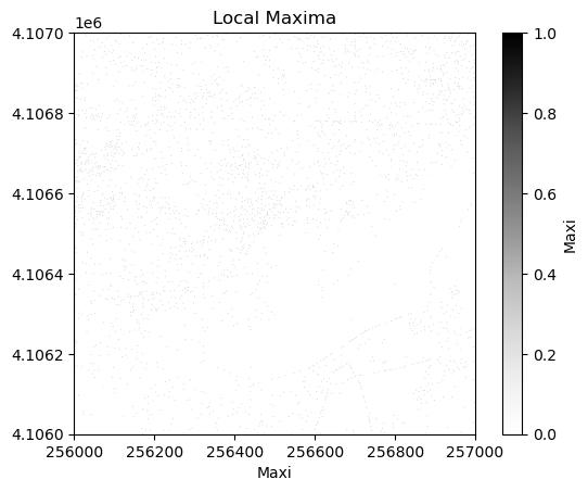
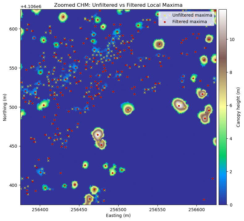
Looking at the overlap between the tree crowns and the local maxima from each method, you can see that filtering improves the results.
# Zoomed CHM section with unfiltered vs filtered local maxima overlay
from mpl_toolkits.axes_grid1 import make_axes_locatable

n_rows, n_cols = chm_array_smooth.shape

# Define a small window around the center of the tile
win_rows = min(250, n_rows)
win_cols = min(250, n_cols)
r0 = max(0, (n_rows // 2) - (win_rows // 2))
c0 = max(0, (n_cols // 2) - (win_cols // 2))
r1 = min(n_rows, r0 + win_rows)
c1 = min(n_cols, c0 + win_cols)

chm_zoom = chm_array_smooth[r0:r1, c0:c1]
local_zoom_filtered = local_maxi[r0:r1, c0:c1]
local_zoom_unfiltered = local_maxi_unfiltered[r0:r1, c0:c1]

# Use rasterio transform to get the true map extent for this zoom window
transform = chm_profile["transform"]
left, top = rio.transform.xy(transform, r0, c0, offset='ul')
right, bottom = rio.transform.xy(transform, r1 - 1, c1 - 1, offset='lr')
zoom_extent = (left, right, bottom, top)

# Convert local maxima row/col indices to map x/y for plotting
peak_rows_filtered, peak_cols_filtered = np.where(local_zoom_filtered)
peak_x_filtered, peak_y_filtered = rio.transform.xy(
    transform,
    peak_rows_filtered + r0,
    peak_cols_filtered + c0,
    offset='center'
    )

peak_rows_unfiltered, peak_cols_unfiltered = np.where(local_zoom_unfiltered)
peak_x_unfiltered, peak_y_unfiltered = rio.transform.xy(
    transform,
    peak_rows_unfiltered + r0,
    peak_cols_unfiltered + c0,
    offset='center'
    )

fig, ax = plt.subplots(figsize=(8, 8))
im = ax.imshow(chm_zoom, cmap='terrain', extent=zoom_extent, origin='upper')

if len(peak_x_unfiltered) > 0:
    ax.scatter(
        peak_x_unfiltered, peak_y_unfiltered, s=18, marker='x', c='yellow',
        linewidths=0.7, label='Unfiltered maxima'
        )
if len(peak_x_filtered) > 0:
    ax.scatter(
        peak_x_filtered, peak_y_filtered, s=14, c='red', edgecolors='black',
        linewidths=0.3, label='Filtered maxima'
        )

ax.set_title('Zoomed CHM: Unfiltered vs Filtered Local Maxima')
ax.set_xlabel('Easting (m)')
ax.set_ylabel('Northing (m)')
ax.legend(loc='upper right')

# Create a colorbar axis matched to the plot's y-axis height
divider = make_axes_locatable(ax)
cax = divider.append_axes('right', size='4%', pad=0.08)
fig.colorbar(im, cax=cax, label='Canopy height (m)')

plt.tight_layout()
#Identify all the maximum points
markers = ndi.label(local_maxi)[0]
Next, create a mask layer of all of the vegetation points so that the watershed segmentation will only occur on the trees and not extend into the surrounding ground points. Since 0 represent ground points in the CHM, setting the mask to 1 where the CHM is not zero will define the mask
#Create a CHM mask so the segmentation will only occur on the trees
chm_mask = chm_array_smooth
chm_mask[chm_array_smooth != 0] = 1
Watershed segmentation
As in a river system, a watershed is divided by a ridge that divides areas. Here our watershed are the individual tree canopies and the ridge is the delineation between each one.
See Basics of Image Processing - Watershed Segmentation for more information on this algorithm.
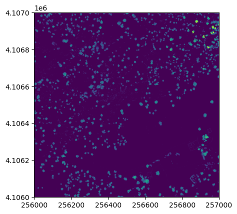
Next, carry out the watershed segmentation. This produces a raster of labels. First, we'll visualize the steps of the watershed segmentation process.
# Create a visualization showing the watershed segmentation process
fig, axes = plt.subplots(1, 2, figsize=(15, 5))

# Panel 1: Smoothed CHM with local maxima (markers)
im1 = axes[0].imshow(chm_array_smooth, cmap='viridis', extent=extent, origin='upper')
axes[0].scatter(chm_bounds.left + np.where(markers)[1] * (chm_bounds.right - chm_bounds.left) / chm_array_smooth.shape[1],
                chm_bounds.top - np.where(markers)[0] * (chm_bounds.top - chm_bounds.bottom) / chm_array_smooth.shape[0],
                c='red', s=30, marker='x', linewidths=2, label='Tree tops (markers)')
axes[0].set_title('Step 1: Smoothed CHM\nwith Tree Top Markers', fontsize=12, fontweight='bold')
axes[0].set_xlabel('X coordinate')
axes[0].set_ylabel('Y coordinate')
axes[0].legend(loc='upper right')
plt.colorbar(im1, ax=axes[0], label='Height (m)')

# Panel 2: CHM with vegetation mask
masked_chm = np.where(chm_mask, chm_array_smooth, np.nan)
im2 = axes[1].imshow(masked_chm, cmap='Greens', extent=extent, origin='upper')
axes[1].set_title('Step 2: Vegetation Mask\n(Algorithm only operates on vegetation)', fontsize=12, fontweight='bold')
axes[1].set_xlabel('X coordinate')
axes[1].set_ylabel('Y coordinate')
plt.colorbar(im2, ax=axes[1], label='Height (m)');
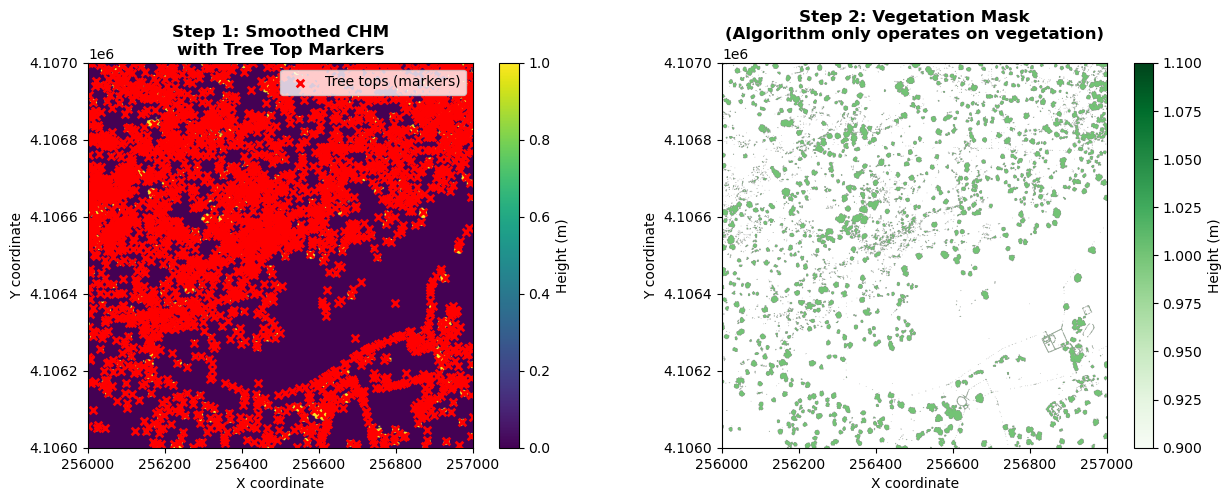
The visualization above shows the first two stages of watershed segmentation: 1. smoothing the CHM with detected tree top markers (red x's), and 2) the vegetation mask, showing only areas with trees included. The third and final step showing the resulting segments are shown after performing the watershed segmentation, in the next cell.
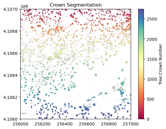
# Perform watershed segmentation
labels = watershed(chm_array_smooth, markers, mask=chm_mask)
labels_for_plot = labels.copy()
labels_for_plot = np.array(labels_for_plot,dtype = np.float32)
labels_for_plot[labels_for_plot==0] = np.nan
max_labels = np.max(labels)
# Plot the segments
plt.figure(4)
plt.imshow(labels_for_plot, cmap='Spectral', extent=extent, origin='upper', vmin=0, vmax=max_labels)
plt.title('Crown Segmentation')
plt.colorbar(label='Tree Crown Number')

plt.savefig(data_path+chm_name[0:-4]+'_Segmentation.png',
            dpi=300,orientation='landscape',
            bbox_inches='tight',pad_inches=0.1)

output_raster(
    os.path.join(data_path, 'labels.tif'),
    labels,
    chm_profile,
    dtype="int32",
    nodata=0
    )
Now collect several properties of the individual trees that will be used as predictor variables.
#Get the properties of each segment
tree_properties = regionprops(labels,chm_array)
Now we will get the predictor variables to match the (soon to be loaded) training data using the get_predictors function defined above. The first column is the segment ID, and the rest are the predictor variables, namely the tree area (pixels), major_axis_length, maximum height, minimum height, height percentiles (p50, p60, p70), and crown geometric volume percentiles (full and percentiles 50, 60, and 70).
predictors_chm = np.array([get_predictors(tree, chm_array, labels) for tree in tree_properties])
X = predictors_chm[:,1:]
tree_ids = predictors_chm[:,0]
np.shape(predictors_chm)
(2749, 12)
We now read the training data directly from GitHub. The CSV contains 12 columns: biomass (the target variable), followed by 11 predictor variables: area, major_axis_length, max_height, min_height, p50, p60, p70, full_crown, crown50, crown60, and crown70. Field-validated tree diameter (DBH) values are used to compute biomass using the formulas from Jenkins et al. (2003), while the remaining predictors were derived from the CHM by manually delineating tree crowns.
# Read training data from download path
training_data_csv = r'C:\NEON-Data-Skills\tutorials\Python\AOP\Lidar\lidar-applications\lidar-biomass\calc-biomass_py_files\SJER_Biomass_Training.csv'

# Alternatively, read training data directly from GitHub (raw CSV)
# training_data_csv = ('https://raw.githubusercontent.com/NEONScience/NEON-Data-Skills/'
#                      'main/tutorials/Python/AOP/Lidar/lidar-applications/'
#                      'lidar-biomass/calc-biomass_py_files/SJER_Biomass_Training.csv')

training_df = pd.read_csv(training_data_csv)

# Build per-column rounding: 0 dp for integer columns, 1 dp for float columns
decimals = {c: (0 if training_df[c].dtype == np.int64 else 1) for c in training_df.columns}

# Preview the data
print('Shape:', training_df.shape)
print()
print('First 5 rows:')
display(training_df.head().round(decimals))
print()
print('Summary statistics:')
display(training_df.describe().round(1))

# Extract numpy arrays for the model
biomass = training_df['biomass'].values
biomass_predictors = training_df.drop(columns=['biomass']).values
Shape: (42, 12)

First 5 rows:
| biomass | area | major_axis_length | max_height | min_height | p50 | p60 | p70 | full_crown | crown50 | crown60 | crown70 | |
|---|---|---|---|---|---|---|---|---|---|---|---|---|
| 0 | 14.2 | 23 | 5.6 | 9 | 5.4 | 8.2 | 8.4 | 8.5 | 54.1 | 48.7 | 50.5 | 51.5 |
| 1 | 7643.4 | 47 | 10.9 | 12 | 6.7 | 10.4 | 10.7 | 10.8 | 159.0 | 146.0 | 151.0 | 154.0 |
| 2 | 889.0 | 16 | 12.4 | 11 | 7.0 | 9.8 | 10.1 | 10.2 | 39.5 | 34.8 | 37.0 | 37.3 |
| 3 | 456.9 | 26 | 10.3 | 11 | 5.8 | 8.6 | 9.0 | 9.2 | 68.6 | 55.5 | 60.8 | 62.6 |
| 4 | 296.7 | 5 | 11.8 | 11 | 8.3 | 10.6 | 10.7 | 10.8 | 9.4 | 8.4 | 8.6 | 8.7 |
Summary statistics:
| biomass | area | major_axis_length | max_height | min_height | p50 | p60 | p70 | full_crown | crown50 | crown60 | crown70 | |
|---|---|---|---|---|---|---|---|---|---|---|---|---|
| count | 42.0 | 42.0 | 42.0 | 42.0 | 42.0 | 42.0 | 42.0 | 42.0 | 42.0 | 42.0 | 42.0 | 42.0 |
| mean | 2644.0 | 33.5 | 8.4 | 9.2 | 5.1 | 7.5 | 7.8 | 8.0 | 99.9 | 85.6 | 90.1 | 93.2 |
| std | 4851.6 | 29.3 | 3.4 | 3.6 | 1.8 | 2.7 | 2.8 | 2.9 | 129.5 | 113.3 | 118.5 | 122.2 |
| min | 14.2 | 3.0 | 3.6 | 5.0 | 2.1 | 2.8 | 2.9 | 3.3 | 1.4 | 0.3 | 0.5 | 0.8 |
| 25% | 240.1 | 15.2 | 6.1 | 7.0 | 4.0 | 5.7 | 5.8 | 6.0 | 26.2 | 23.5 | 24.0 | 24.7 |
| 50% | 659.4 | 23.0 | 7.5 | 8.5 | 5.0 | 7.0 | 7.2 | 7.3 | 47.4 | 38.2 | 41.0 | 42.3 |
| 75% | 2791.3 | 41.2 | 10.7 | 11.0 | 5.7 | 8.6 | 9.0 | 9.2 | 88.4 | 72.2 | 78.4 | 82.8 |
| max | 25968.4 | 118.0 | 18.2 | 21.0 | 11.8 | 15.5 | 16.0 | 16.5 | 627.0 | 553.0 | 574.0 | 591.0 |
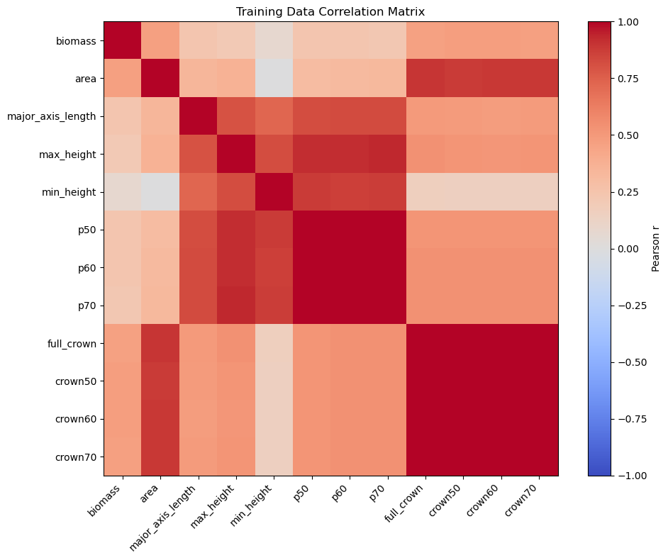
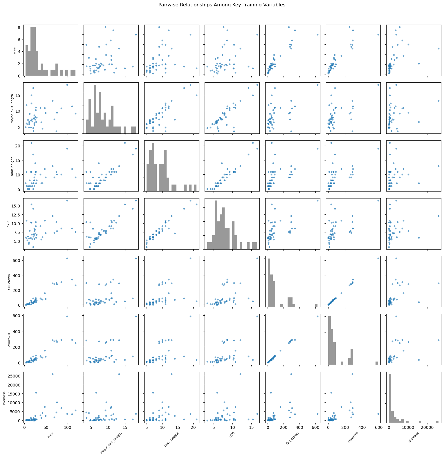
Let's inspect the training data by making some pairwise plots.
# Inspect pairwise relationships among training-data columns
column_names = training_df.columns.tolist()

# Summary table
summary = training_df.describe().round(1)
print('Column summary (min, max, mean, std):')
for name in column_names:
    mn = summary.loc['min', name]
    mx = summary.loc['max', name]
    mu = summary.loc['mean', name]
    sd = summary.loc['std', name]
    print(f'{name:>16s}: min={mn:10.1f}, max={mx:10.1f}, mean={mu:10.1f}, std={sd:10.1f}')

# Plot 1: correlation heatmap (all columns)
corr = training_df.corr(numeric_only=True)
fig, ax = plt.subplots(figsize=(10, 8))
im = ax.imshow(corr, cmap='coolwarm', vmin=-1, vmax=1)
ax.set_xticks(np.arange(len(corr.columns)))
ax.set_yticks(np.arange(len(corr.columns)))
ax.set_xticklabels(corr.columns, rotation=45, ha='right')
ax.set_yticklabels(corr.columns)
ax.set_title('Training Data Correlation Matrix')
plt.colorbar(im, ax=ax, label='Pearson r')
plt.tight_layout()

# Plot 2: scatter matrix style plot (key variables)
plot_columns = [
    'area', 'major_axis_length', 'max_height', 'p70',
    'full_crown', 'crown70', 'biomass'
    ]
plot_df = training_df[plot_columns]

n = len(plot_columns)
fig, axes = plt.subplots(n, n, figsize=(2.2 * n, 2.2 * n), squeeze=False)
for i in range(n):
    for j in range(n):
        ax = axes[i, j]
        if i == j:
            ax.hist(plot_df.iloc[:, j], bins=20, color='gray', alpha=0.8)
        else:
            ax.scatter(plot_df.iloc[:, j], plot_df.iloc[:, i], s=10, alpha=0.6, color='tab:blue')

        if i == n - 1:
            ax.set_xlabel(plot_columns[j], fontsize=8, rotation=45)
        else:
            ax.set_xticklabels([])
        if j == 0:
            ax.set_ylabel(plot_columns[i], fontsize=8)
        else:
            ax.set_yticklabels([])

fig.suptitle('Pairwise Relationships Among Key Training Variables', y=1.02)
plt.tight_layout()
Column summary (min, max, mean, std):
         biomass: min=      14.2, max=   25968.4, mean=    2644.0, std=    4851.6
            area: min=       3.0, max=     118.0, mean=      33.5, std=      29.3
major_axis_length: min=       3.6, max=      18.2, mean=       8.4, std=       3.4
      max_height: min=       5.0, max=      21.0, mean=       9.2, std=       3.6
      min_height: min=       2.1, max=      11.8, mean=       5.1, std=       1.8
             p50: min=       2.8, max=      15.5, mean=       7.5, std=       2.7
             p60: min=       2.9, max=      16.0, mean=       7.8, std=       2.8
             p70: min=       3.3, max=      16.5, mean=       8.0, std=       2.9
      full_crown: min=       1.4, max=     627.0, mean=      99.9, std=     129.5
         crown50: min=       0.3, max=     553.0, mean=      85.6, std=     113.3
         crown60: min=       0.5, max=     574.0, mean=      90.1, std=     118.5
         crown70: min=       0.8, max=     591.0, mean=      93.2, std=     122.2
Random Forest classifiers
We can then define parameters of the Random Forest classifier and fit the predictor variables from the training data to the Biomass estimates.
#Define parameters for the Random Forest Regressor
max_depth = 30

#Define regressor settings
regr_rf = RandomForestRegressor(max_depth=max_depth, random_state=2)

#Fit the biomass to regressor variables
regr_rf.fit(biomass_predictors,biomass)
We will now apply the Random Forest model to the predictor variables to estimate biomass
#Apply the model to the predictors
estimated_biomass = regr_rf.predict(X)
To output a raster, pre-allocate (copy) an array from the labels raster, then cycle through the segments and assign the biomass estimate to each individual tree segment.
#Set an out raster with the same size as the labels
biomass_map =  np.array((labels),dtype=float)
#Assign the appropriate biomass to the labels
biomass_map[biomass_map==0] = np.nan
for tree_id, biomass_of_tree_id in zip(tree_ids, estimated_biomass):
    biomass_map[biomass_map == tree_id] = biomass_of_tree_id
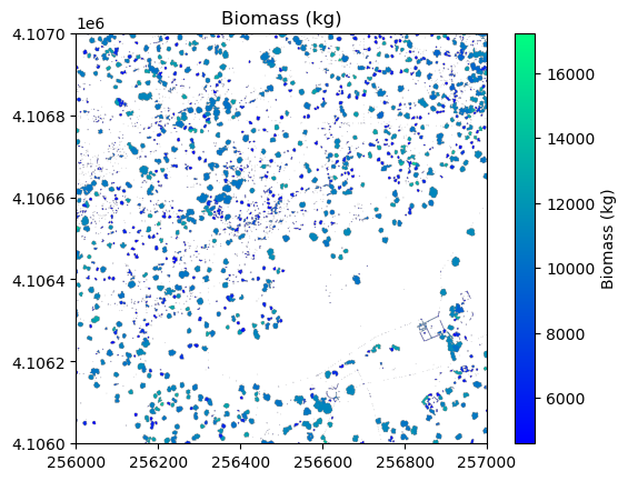
Calculate Biomass
Collect some of the biomass statistics and then plot the results and save an output geotiff.
#Get biomass stats for plotting
mean_biomass = np.mean(estimated_biomass)
std_biomass = np.std(estimated_biomass)
min_biomass = np.min(estimated_biomass)
sum_biomass = np.sum(estimated_biomass)

print('Sum of above ground biomass (AGB) is',round(sum_biomass,1),'kg')

# Plot the biomass
plt.figure(5)
plt.imshow(
    biomass_map,
    cmap='winter',
    extent=extent,
    origin='upper',
    vmin=min_biomass + std_biomass,
    vmax=mean_biomass + std_biomass * 3
    )
plt.title('Biomass (kg)')
plt.colorbar(label='Biomass (kg)')

# Save the biomass figure; use the same name as the original file, but replace CHM with Biomass
plt.savefig(os.path.join(data_path,chm_name.replace('CHM.tif','Biomass.png')),
            dpi=300,orientation='landscape',
            bbox_inches='tight',
            pad_inches=0.1)

# Write biomass geotiff with rasterio
output_raster(
    os.path.join(data_path, chm_name.replace('CHM.tif','Biomass.tif')),
    biomass_map,
    chm_profile,
    dtype="float32",
    nodata=np.nan
    )
Sum of above ground biomass (AGB) is 10515682.7 kg