This tutorial will overview the key attributes of a raster object, including spatial extent, resolution and coordinate reference system. When working within a GIS system often these attributes are accounted for. However, it is important to be more familiar with them when working in non-GUI environments such as R or even Python.

In order to correctly spatially reference a raster that is not already georeferenced, you will also need to identify:

1. The lower left hand corner coordinates of the raster.
2. The number of columns and rows that the raster dataset contains.

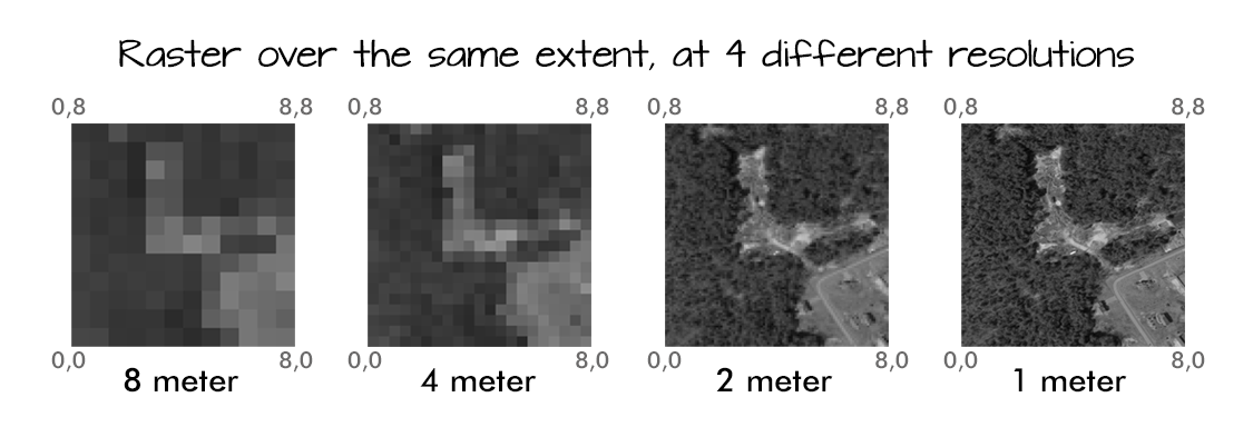
Spatial Resolution

A raster consists of a series of pixels, each with the same dimensions and shape. In the case of rasters derived from airborne sensors, each pixel represents an area of space on the Earth's surface. The size of the area on the surface that each pixel covers is known as the spatial resolution of the image. For instance, an image that has a 1 m spatial resolution means that each pixel in the image represents a 1 m x 1 m area.

Load the Data

Let's open up a raster in R to see how the attributes are stored. We are going to work with a Digital Terrain Model from the San Joaquin Experimental Range in California.

# load packages 
library(raster)  
library(rgdal)

# set working directory to data folder
#setwd("pathToDirHere")
wd <- ("~/Git/data/")
setwd(wd)

# Load raster in an R object called 'DEM'
DEM <- raster(paste0(wd, "NEON-DS-Field-Site-Spatial-Data/SJER/DigitalTerrainModel/SJER2013_DTM.tif"))  


# View raster attributes 
DEM

## class      : RasterLayer 
## dimensions : 5060, 4299, 21752940  (nrow, ncol, ncell)
## resolution : 1, 1  (x, y)
## extent     : 254570, 258869, 4107302, 4112362  (xmin, xmax, ymin, ymax)
## crs        : +proj=utm +zone=11 +datum=WGS84 +units=m +no_defs 
## source     : /Users/olearyd/Git/data/NEON-DS-Field-Site-Spatial-Data/SJER/DigitalTerrainModel/SJER2013_DTM.tif 
## names      : SJER2013_DTM

Note that this raster (in GeoTIFF format) already has an extent, resolution, and CRS defined. The resolution in both x and y directions is 1. The CRS tells us that the x,y units of the data are meters (m).

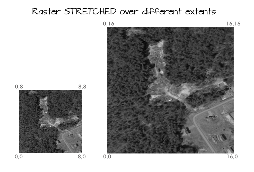
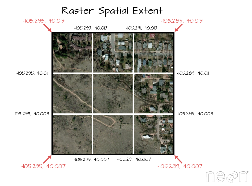
Spatial Extent

The spatial extent of a raster, represents the "X, Y" coordinates of the corners of the raster in geographic space. This information, in addition to the cell size or spatial resolution, tells the program how to place or render each pixel in 2 dimensional space. Tools like R, using supporting packages such as rgdal and associated raster tools have functions that allow you to view and define the extent of a new raster.

# View the extent of the raster
DEM@extent

## class      : Extent 
## xmin       : 254570 
## xmax       : 258869 
## ymin       : 4107302 
## ymax       : 4112362

Calculating Raster Extent

Extent and spatial resolution are closely connected. To calculate the extent of a raster, we first need the bottom left hand (X,Y) coordinate of the raster. In the case of the UTM coordinate system which is in meters, to calculate the raster's extent, we can add the number of columns and rows to the X,Y corner coordinate location of the raster, multiplied by the resolution (the pixel size) of the raster.

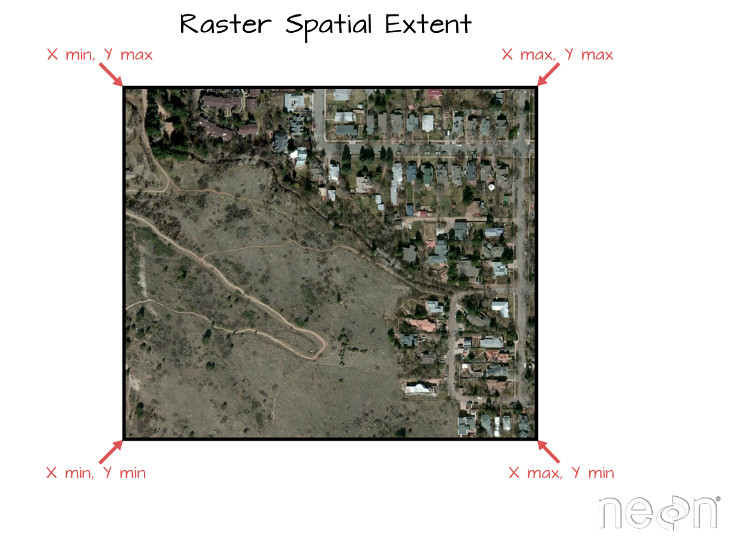
<figcaption>To be located geographically, a raster's location needs to be 
defined in geographic space (i.e., on a spatial grid). The spatial extent 
defines the four corners of a raster within a given coordinate reference 
system. Source: National Ecological Observatory Network. </figcaption>

Let's explore that next, using a blank raster that we create.

# create a raster from the matrix - a "blank" raster of 4x4
myRaster1 <- raster(nrow=4, ncol=4)

# assign "data" to raster: 1 to n based on the number of cells in the raster
myRaster1[]<- 1:ncell(myRaster1)

# view attributes of the raster
myRaster1

## class      : RasterLayer 
## dimensions : 4, 4, 16  (nrow, ncol, ncell)
## resolution : 90, 45  (x, y)
## extent     : -180, 180, -90, 90  (xmin, xmax, ymin, ymax)
## crs        : +proj=longlat +datum=WGS84 +no_defs 
## source     : memory
## names      : layer 
## values     : 1, 16  (min, max)

# is the CRS defined?
myRaster1@crs

## CRS arguments: +proj=longlat +datum=WGS84 +no_defs

Wait, why is the CRS defined on this new raster? This is the default values for something created with the raster() function if nothing is defined.

Let's get back to looking at more attributes.

# what is the raster extent?
myRaster1@extent

## class      : Extent 
## xmin       : -180 
## xmax       : 180 
## ymin       : -90 
## ymax       : 90

# plot raster
plot(myRaster1, main="Raster with 16 pixels")

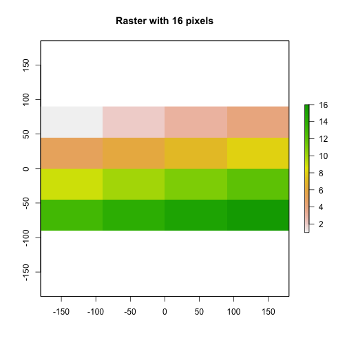
Here we see our raster with the value of 1 to 16 in each pixel.

We can resample the raster as well to adjust the resolution. If we want a higher resolution raster, we will apply a grid with more pixels within the same extent. If we want a lower resolution raster, we will apply a grid with fewer pixels within the same extent.

One way to do this is to create a raster of the resolution you want and then resample() your original raster. The resampling will be done for either nearest neighbor assignments (for categorical data) or bilinear interpolation (for numerical data).

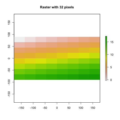
## HIGHER RESOLUTION
# Create 32 pixel raster
myRaster2 <- raster(nrow=8, ncol=8)

# resample 16 pix raster with 32 pix raster
# use bilinear interpolation with our numeric data
myRaster2 <- resample(myRaster1, myRaster2, method='bilinear')

# notice new dimensions, resolution, & min/max 
myRaster2

## class      : RasterLayer 
## dimensions : 8, 8, 64  (nrow, ncol, ncell)
## resolution : 45, 22.5  (x, y)
## extent     : -180, 180, -90, 90  (xmin, xmax, ymin, ymax)
## crs        : +proj=longlat +datum=WGS84 +no_defs 
## source     : memory
## names      : layer 
## values     : -0.25, 17.25  (min, max)

# plot 
plot(myRaster2, main="Raster with 32 pixels")

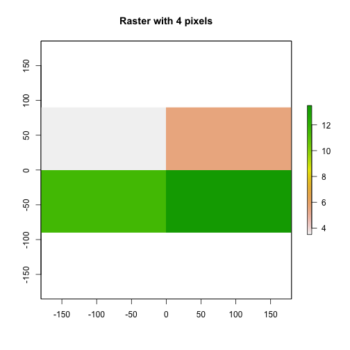
## LOWER RESOLUTION
myRaster3 <- raster(nrow=2, ncol=2)
myRaster3 <- resample(myRaster1, myRaster3, method='bilinear')
myRaster3

## class      : RasterLayer 
## dimensions : 2, 2, 4  (nrow, ncol, ncell)
## resolution : 180, 90  (x, y)
## extent     : -180, 180, -90, 90  (xmin, xmax, ymin, ymax)
## crs        : +proj=longlat +datum=WGS84 +no_defs 
## source     : memory
## names      : layer 
## values     : 3.5, 13.5  (min, max)

plot(myRaster3, main="Raster with 4 pixels")

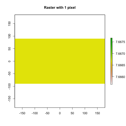
## SINGLE PIXEL RASTER
myRaster4 <- raster(nrow=1, ncol=1)
myRaster4 <- resample(myRaster1, myRaster4, method='bilinear')
myRaster4

## class      : RasterLayer 
## dimensions : 1, 1, 1  (nrow, ncol, ncell)
## resolution : 360, 180  (x, y)
## extent     : -180, 180, -90, 90  (xmin, xmax, ymin, ymax)
## crs        : +proj=longlat +datum=WGS84 +no_defs 
## source     : memory
## names      : layer 
## values     : 7.666667, 7.666667  (min, max)

plot(myRaster4, main="Raster with 1 pixel")

To more easily compare them, let's create a graphic layout with 4 rasters in it. Notice that each raster has the same extent but each a different resolution because it has a different number of pixels spread out over the same extent.

# change graphical parameter to 2x2 grid
par(mfrow=c(2,2))

# arrange plots in order you wish to see them
plot(myRaster2, main="Raster with 32 pixels")
plot(myRaster1, main="Raster with 16 pixels")
plot(myRaster3, main="Raster with 4 pixels")
plot(myRaster4, main="Raster with 2 pixels")

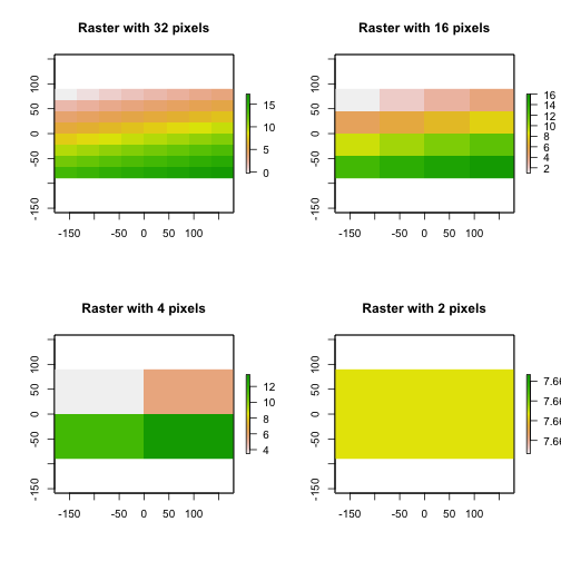
# change graphical parameter back to 1x1 
par(mfrow=c(1,1))

Extent & Coordinate Reference Systems

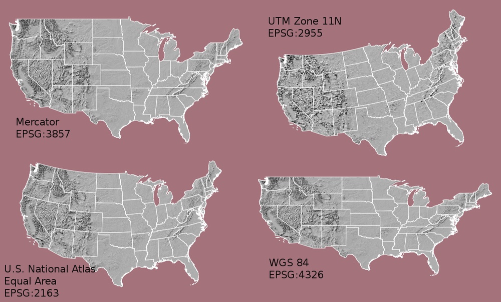
Coordinate Reference System & Projection Information

A spatial reference system (SRS) or coordinate reference system (CRS) is a coordinate-based local, regional or global system used to locate geographical entities. -- Wikipedia

The earth is round. This is not an new concept by any means, however we need to remember this when we talk about coordinate reference systems associated with spatial data. When we make maps on paper or on a computer screen, we are moving from a 3 dimensional space (the globe) to 2 dimensions (our computer screens or a piece of paper). To keep this short, the projection of a dataset relates to how the data are "flattened" in geographic space so our human eyes and brains can make sense of the information in 2 dimensions.

The projection refers to the mathematical calculations performed to "flatten the data" in into 2D space. The coordinate system references to the x and y coordinate space that is associated with the projection used to flatten the data. If you have the same dataset saved in two different projections, these two files won't line up correctly when rendered together.

Read more about projections.

How Map Projections Can Fool the Eye

Check out this short video, by Buzzfeed, highlighting how map projections can make continents seems proportionally larger or smaller than they actually are!

What Makes Spatial Data Line Up On A Map?

There are lots of great resources that describe coordinate reference systems and projections in greater detail. However, for the purposes of this activity, what is important to understand is that data from the same location but saved in different projections will not line up in any GIS or other program. Thus it's important when working with spatial data in a program like R or Python to identify the coordinate reference system applied to the data, and to grab that information and retain it when you process / analyze the data.

For a library of CRS information: A great online library of CRS information.

CRS proj4 Strings

The rgdal package has all the common ESPG codes with proj4string built in. We can see them by creating an object of the function make_ESPG().

# make sure you loaded rgdal package at the top of your script

# create an object with all ESPG codes
epsg = make_EPSG()

# use View(espg) to see the full table - doesn't render on website well
#View(epsg)

# View top 5 entries
head(epsg, 5)

##   code   note                                                   prj4
## 1 3819 HD1909         +proj=longlat +ellps=bessel +no_defs +type=crs
## 2 3821  TWD67        +proj=longlat +ellps=aust_SA +no_defs +type=crs
## 3 3822  TWD97 +proj=geocent +ellps=GRS80 +units=m +no_defs +type=crs
## 4 3823  TWD97          +proj=longlat +ellps=GRS80 +no_defs +type=crs
## 5 3824  TWD97          +proj=longlat +ellps=GRS80 +no_defs +type=crs
##   prj_method
## 1     (null)
## 2     (null)
## 3     (null)
## 4     (null)
## 5     (null)

Define the extent

In the above raster example, we created several simple raster objects in R. R defaulted to a global lat/long extent. We can define the exact extent that we need to use too.

Let's create a new raster with the same projection as our original DEM. We know that our data are in UTM zone 11N. For the sake of this exercise, let say we want to create a raster with the left hand corner coordinate at:

• xmin = 254570
• ymin = 4107302

The resolution of this new raster will be 1 meter and we will be working in UTM (meters). First, let's set up the raster.

# create 10x20 matrix with values 1-8. 
newMatrix  <- (matrix(1:8, nrow = 10, ncol = 20))

# convert to raster
rasterNoProj <- raster(newMatrix)
rasterNoProj

## class      : RasterLayer 
## dimensions : 10, 20, 200  (nrow, ncol, ncell)
## resolution : 0.05, 0.1  (x, y)
## extent     : 0, 1, 0, 1  (xmin, xmax, ymin, ymax)
## crs        : NA 
## source     : memory
## names      : layer 
## values     : 1, 8  (min, max)

Now we can define the new raster's extent by defining the lower left corner of the raster.

## Define the xmin and ymin (the lower left hand corner of the raster)

# 1. define xMin & yMin objects.
xMin = 254570
yMin = 4107302

# 2. grab the cols and rows for the raster using @ncols and @nrows
rasterNoProj@ncols

## [1] 20

rasterNoProj@nrows

## [1] 10

# 3. raster resolution
res <- 1.0

# 4. add the numbers of cols and rows to the x,y corner location, 
# result = we get the bounds of our raster extent. 
xMax <- xMin + (rasterNoProj@ncols * res)
yMax <- yMin + (rasterNoProj@nrows * res)

# 5.create a raster extent class
rasExt <- extent(xMin,xMax,yMin,yMax)
rasExt

## class      : Extent 
## xmin       : 254570 
## xmax       : 254590 
## ymin       : 4107302 
## ymax       : 4107312

# 6. apply the extent to our raster
rasterNoProj@extent <- rasExt

# Did it work? 
rasterNoProj

## class      : RasterLayer 
## dimensions : 10, 20, 200  (nrow, ncol, ncell)
## resolution : 1, 1  (x, y)
## extent     : 254570, 254590, 4107302, 4107312  (xmin, xmax, ymin, ymax)
## crs        : NA 
## source     : memory
## names      : layer 
## values     : 1, 8  (min, max)

# or view extent only
rasterNoProj@extent

## class      : Extent 
## xmin       : 254570 
## xmax       : 254590 
## ymin       : 4107302 
## ymax       : 4107312

Now we have an extent associated with our raster which places it in space!

# plot new raster
plot(rasterNoProj, main="Raster in UTM coordinates, 1 m resolution")

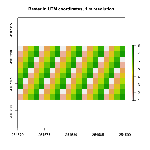
Notice that the coordinates show up on our plot now.

Define Projection of a Raster

We can define the projection of a raster that has a known CRS already. Sometimes we download data that have projection information associated with them but the CRS is not defined either in the GeoTIFF tags or in the raster itself. If this is the case, we can simply assign the raster the correct projection.

Be careful doing this - it is not the same thing as reprojecting your data.

Let's define the projection for our newest raster using the DEM raster that already has defined CRS. NOTE: in this case we have to know that our raster is in this projection already so we don't run the risk of assigning the wrong projection to the data.

# view CRS from raster of interest
rasterNoProj@crs

## CRS arguments: NA

# view the CRS of our DEM object.
DEM@crs

## CRS arguments:
##  +proj=utm +zone=11 +datum=WGS84 +units=m +no_defs

# define the CRS using a CRS of another raster
rasterNoProj@crs <- DEM@crs

# look at the attributes
rasterNoProj

## class      : RasterLayer 
## dimensions : 10, 20, 200  (nrow, ncol, ncell)
## resolution : 1, 1  (x, y)
## extent     : 254570, 254590, 4107302, 4107312  (xmin, xmax, ymin, ymax)
## crs        : +proj=utm +zone=11 +datum=WGS84 +units=m +no_defs 
## source     : memory
## names      : layer 
## values     : 1, 8  (min, max)

# view just the crs
rasterNoProj@crs

## CRS arguments:
##  +proj=utm +zone=11 +datum=WGS84 +units=m +no_defs

IMPORTANT: the above code does not reproject the raster. It simply defines the Coordinate Reference System based upon the CRS of another raster. If you want to actually change the CRS of a raster, you need to use the projectRaster function.

## Challenge Example Code 

# set latLong
latLong <- data.frame(longitude=seq( 0,10,1), latitude=seq( 0,10,1))

# make spatial points dataframe, which will have a spatial extent
sp <- SpatialPoints( latLong[ c("longitude" , "latitude") ], proj4string = CRS("+proj=longlat +datum=WGS84") )

# make raster based on the extent of your data
r <- raster(nrow=5, ncol=5, extent( sp ) )

r[]  <- 1
r[]  <- sample(0:50,25)
r

## class      : RasterLayer 
## dimensions : 5, 5, 25  (nrow, ncol, ncell)
## resolution : 2, 2  (x, y)
## extent     : 0, 10, 0, 10  (xmin, xmax, ymin, ymax)
## crs        : NA 
## source     : memory
## names      : layer 
## values     : 3, 50  (min, max)

Reprojecting Data

If you run into multiple spatial datasets with varying projections, you can always reproject the data so that they are all in the same projection. Python and R both have reprojection tools that perform this task.

# reproject raster data from UTM to CRS of Lat/Long WGS84
reprojectedData1 <- projectRaster(rasterNoProj, 
                                 crs="+proj=longlat +ellps=WGS84 +datum=WGS84 +no_defs ")

# note that the extent has been adjusted to account for the NEW crs
reprojectedData1@crs

## CRS arguments: +proj=longlat +datum=WGS84 +no_defs

reprojectedData1@extent

## class      : Extent 
## xmin       : -119.761 
## xmax       : -119.7607 
## ymin       : 37.07988 
## ymax       : 37.08

# note the range of values in the output data
reprojectedData1

## class      : RasterLayer 
## dimensions : 13, 22, 286  (nrow, ncol, ncell)
## resolution : 1.12e-05, 9e-06  (x, y)
## extent     : -119.761, -119.7607, 37.07988, 37.08  (xmin, xmax, ymin, ymax)
## crs        : +proj=longlat +datum=WGS84 +no_defs 
## source     : memory
## names      : layer 
## values     : 0.64765, 8.641957  (min, max)

# use nearest neighbor interpolation method to ensure that the values stay the same
reprojectedData2 <- projectRaster(rasterNoProj, 
                                 crs="+proj=longlat +ellps=WGS84 +datum=WGS84 +no_defs ", 
                                 method = "ngb")


# note that the min and max values have now been forced to stay within the same range.
reprojectedData2

## class      : RasterLayer 
## dimensions : 13, 22, 286  (nrow, ncol, ncell)
## resolution : 1.12e-05, 9e-06  (x, y)
## extent     : -119.761, -119.7607, 37.07988, 37.08  (xmin, xmax, ymin, ymax)
## crs        : +proj=longlat +datum=WGS84 +no_defs 
## source     : memory
## names      : layer 
## values     : 1, 8  (min, max)

This activity will walk you through the fundamental principles of working with raster data in R.

What is Raster Data?

Raster or "gridded" data are data that are saved in pixels. In the spatial world, each pixel represents an area on the Earth's surface. For example in the raster below, each pixel represents a particular land cover class that would be found in that location in the real world.

More on rasters in the The Relationship Between Raster Resolution, Spatial extent & Number of Pixels tutorial.

To work with rasters in R, we need two key packages, sp and raster. To install the raster package you can use install.packages('raster'). When you install the raster package, sp should also install. Also install the rgdal package install.packages('rgdal'). Among other things, rgdal will allow us to export rasters to GeoTIFF format.

Once installed we can load the packages and start working with raster data.

# load the raster, sp, and rgdal packages
library(raster)
library(sp)
library(rgdal)

# set working directory to data folder
#setwd("pathToDirHere")
wd <- ("~/Git/data/")
setwd(wd)

Next, let's load a raster containing elevation data into our environment. And look at the attributes.

# load raster in an R object called 'DEM'
DEM <- raster(paste0(wd, "NEON-DS-Field-Site-Spatial-Data/SJER/DigitalTerrainModel/SJER2013_DTM.tif"))

# look at the raster attributes. 
DEM

## class      : RasterLayer 
## dimensions : 5060, 4299, 21752940  (nrow, ncol, ncell)
## resolution : 1, 1  (x, y)
## extent     : 254570, 258869, 4107302, 4112362  (xmin, xmax, ymin, ymax)
## crs        : +proj=utm +zone=11 +datum=WGS84 +units=m +no_defs 
## source     : /Users/olearyd/Git/data/NEON-DS-Field-Site-Spatial-Data/SJER/DigitalTerrainModel/SJER2013_DTM.tif 
## names      : SJER2013_DTM

Notice a few things about this raster.

• dimensions: the "size" of the file in pixels

• nrow, ncol: the number of rows and columns in the data (imagine a spreadsheet or a matrix).
• ncells: the total number of pixels or cells that make up the raster.

• resolution: the size of each pixel (in meters in this case). 1 meter pixels means that each pixel represents a 1m x 1m area on the earth's surface.
• extent: the spatial extent of the raster. This value will be in the same coordinate units as the coordinate reference system of the raster.
• coord ref: the coordinate reference system string for the raster. This raster is in UTM (Universal Trans Mercator) zone 11 with a datum of WGS 84. More on UTM here.

Work with Rasters in R

Now that we have the raster loaded into R, let's grab some key raster attributes.

Define Min/Max Values

By default this raster doesn't have the min or max values associated with it's attributes Let's change that by using the setMinMax() function.

# calculate and save the min and max values of the raster to the raster object
DEM <- setMinMax(DEM)

# view raster attributes
DEM

## class      : RasterLayer 
## dimensions : 5060, 4299, 21752940  (nrow, ncol, ncell)
## resolution : 1, 1  (x, y)
## extent     : 254570, 258869, 4107302, 4112362  (xmin, xmax, ymin, ymax)
## crs        : +proj=utm +zone=11 +datum=WGS84 +units=m +no_defs 
## source     : /Users/olearyd/Git/data/NEON-DS-Field-Site-Spatial-Data/SJER/DigitalTerrainModel/SJER2013_DTM.tif 
## names      : SJER2013_DTM 
## values     : 228.1, 518.66  (min, max)

Notice the values is now part of the attributes and shows the min and max values for the pixels in the raster. What these min and max values represent depends on what is represented by each pixel in the raster.

You can also view the rasters min and max values and the range of values contained within the pixels.

#Get min and max cell values from raster
#NOTE: this code may fail if the raster is too large
cellStats(DEM, min)

## [1] 228.1

cellStats(DEM, max)

## [1] 518.66

cellStats(DEM, range)

## [1] 228.10 518.66

View CRS

First, let's consider the Coordinate Reference System (CRS).

#view coordinate reference system
DEM@crs

## CRS arguments:
##  +proj=utm +zone=11 +datum=WGS84 +units=m +no_defs

This raster is located in UTM Zone 11.

View Extent

If you want to know the exact boundaries of your raster that is in the extent slot.

# view raster extent
DEM@extent

## class      : Extent 
## xmin       : 254570 
## xmax       : 258869 
## ymin       : 4107302 
## ymax       : 4112362

Raster Pixel Values

We can also create a histogram to view the distribution of values in our raster. Note that the max number of pixels that R will plot by default is 100,000. We can tell it to plot more using the maxpixels attribute. Be careful with this, if your raster is large this can take a long time or crash your program.

Since our raster is a digital elevation model, we know that each pixel contains elevation data about our area of interest. In this case the units are meters.

This is an easy and quick data checking tool. Are there any totally weird values?

# the distribution of values in the raster
hist(DEM, main="Distribution of elevation values", 
     col= "purple", 
     maxpixels=22000000)

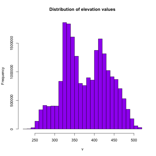
It looks like we have a lot of land around 325m and 425m.

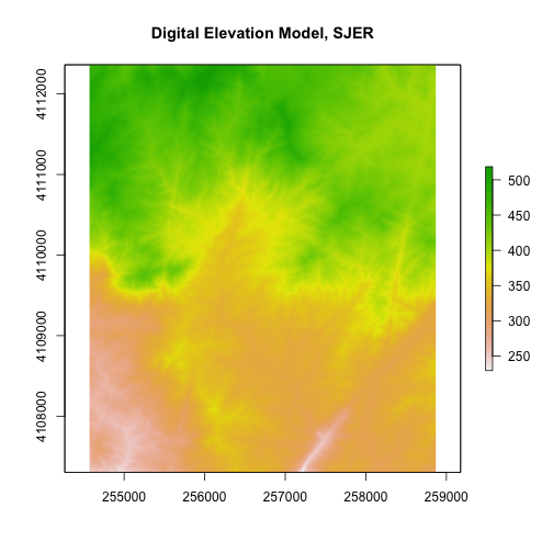
Plot Raster Data

Let's take a look at our raster now that we know a bit more about it. We can do a simple plot with the plot() function.

# plot the raster
# note that this raster represents a small region of the NEON SJER field site
plot(DEM, 
		 main="Digital Elevation Model, SJER") # add title with main

R has an image() function that allows you to control the way a raster is rendered on the screen. The plot() function in R has a base setting for the number of pixels that it will plot (100,000 pixels). The image command thus might be better for rendering larger rasters.

# create a plot of our raster
image(DEM)

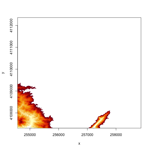
# specify the range of values that you want to plot in the DEM
# just plot pixels between 250 and 300 m in elevation
image(DEM, zlim=c(250,300))

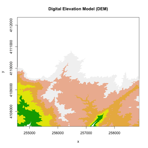
# we can specify the colors too
col <- terrain.colors(5)
image(DEM, zlim=c(250,375), main="Digital Elevation Model (DEM)", col=col)

Plotting with Colors

In the above example. terrain.colors() tells R to create a palette of colors within the terrain.colors color ramp. There are other palettes that you can use as well include rainbow and heat.colors.

• More on color palettes in R here.
• Another good post on colors.
• RColorBrewer is another powerful tool to create sets of colors.

Breaks and Colorbars in R

A digital elevation model (DEM) is an example of a continuous raster. It contains elevation values for a range. For example, elevations values in a DEM might include any set of values between 200 m and 500 m. Given this range, you can plot DEM pixels using a gradient of colors.

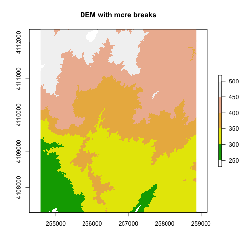
By default, R will assign the gradient of colors uniformly across the full range of values in the data. In our case, our DEM has values between 250 and 500. However, we can adjust the "breaks" which represent the numeric locations where the colors change if we want too.

# add a color map with 5 colors
col=terrain.colors(5)

# add breaks to the colormap (6 breaks = 5 segments)
brk <- c(250, 300, 350, 400, 450, 500)

plot(DEM, col=col, breaks=brk, main="DEM with more breaks")

We can also customize the legend appearance.

# First, expand right side of clipping rectangle to make room for the legend
# turn xpd off
par(xpd = FALSE, mar=c(5.1, 4.1, 4.1, 4.5))

# Second, plot w/ no legend
plot(DEM, col=col, breaks=brk, main="DEM with a Custom (but flipped) Legend", legend = FALSE)

# Third, turn xpd back on to force the legend to fit next to the plot.
par(xpd = TRUE)

# Fourth, add a legend - & make it appear outside of the plot
legend(par()$usr[2], 4110600,
        legend = c("lowest", "a bit higher", "middle ground", "higher yet", "highest"), 
        fill = col)

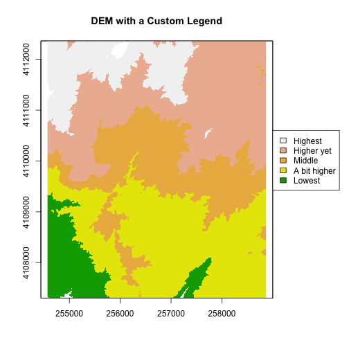
Notice that the legend is in reverse order in the previous plot. Let’s fix that. We need to both reverse the order we have the legend laid out and reverse the the color fill with the rev() colors.

# Expand right side of clipping rect to make room for the legend
par(xpd = FALSE,mar=c(5.1, 4.1, 4.1, 4.5))
#DEM with a custom legend
plot(DEM, col=col, breaks=brk, main="DEM with a Custom Legend",legend = FALSE)
#turn xpd back on to force the legend to fit next to the plot.
par(xpd = TRUE)

#add a legend - but make it appear outside of the plot
legend( par()$usr[2], 4110600,
        legend = c("Highest", "Higher yet", "Middle","A bit higher", "Lowest"), 
        fill = rev(col))

Try the code again but only make one of the changes -- reverse order or reverse colors-- what happens?

The raster plot now inverts the elevations! This is a good reason to understand your data so that a simple visualization error doesn't have you reversing the slope or some other error.

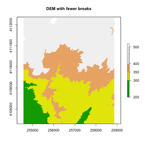
We can add a custom color map with fewer breaks as well.

#add a color map with 4 colors
col=terrain.colors(4)
#add breaks to the colormap (6 breaks = 5 segments)
brk <- c(200, 300, 350, 400,500)
plot(DEM, col=col, breaks=brk, main="DEM with fewer breaks")

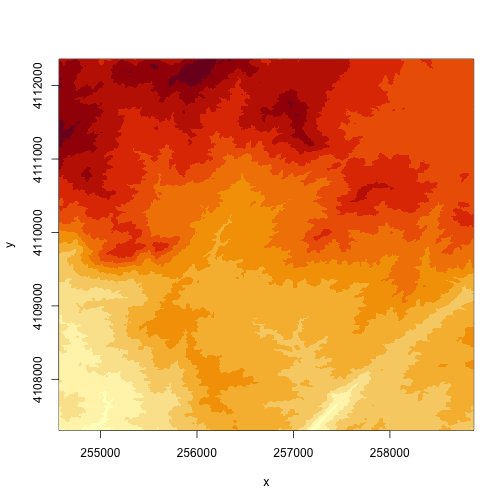
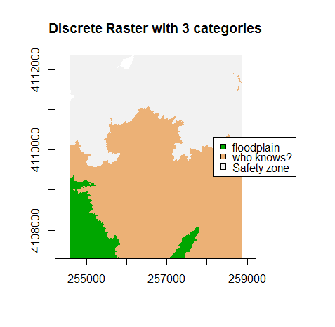
A discrete dataset has a set of unique categories or classes. One example could be land use classes. The example below shows elevation zones generated using the same DEM.

Basic Raster Math

We can also perform calculations on our raster. For instance, we could multiply all values within the raster by 2.

#multiple each pixel in the raster by 2
DEM2 <- DEM * 2

DEM2

## class      : RasterLayer 
## dimensions : 5060, 4299, 21752940  (nrow, ncol, ncell)
## resolution : 1, 1  (x, y)
## extent     : 254570, 258869, 4107302, 4112362  (xmin, xmax, ymin, ymax)
## crs        : +proj=utm +zone=11 +datum=WGS84 +units=m +no_defs 
## source     : memory
## names      : SJER2013_DTM 
## values     : 456.2, 1037.32  (min, max)

#plot the new DEM
plot(DEM2, main="DEM with all values doubled")

Cropping Rasters in R

You can crop rasters in R using different methods. You can crop the raster directly drawing a box in the plot area. To do this, first plot the raster. Then define the crop extent by clicking twice:

1. Click in the UPPER LEFT hand corner where you want the crop box to begin.
2. Click again in the LOWER RIGHT hand corner to define where the box ends.

You'll see a red box on the plot. NOTE that this is a manual process that can be used to quickly define a crop extent.

#plot the DEM
plot(DEM)

#Define the extent of the crop by clicking on the plot
cropbox1 <- drawExtent()

#crop the raster, then plot the new cropped raster
DEMcrop1 <- crop(DEM, cropbox1)

#plot the cropped extent
plot(DEMcrop1)

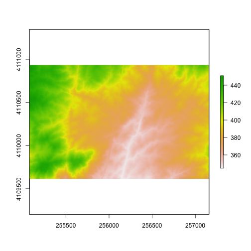
You can also manually assign the extent coordinates to be used to crop a raster. We'll need the extent defined as (xmin, xmax, ymin , ymax) to do this. This is how we'd crop using a GIS shapefile (with a rectangular shape)

#define the crop extent
cropbox2 <-c(255077.3,257158.6,4109614,4110934)
#crop the raster
DEMcrop2 <- crop(DEM, cropbox2)
#plot cropped DEM
plot(DEMcrop2)

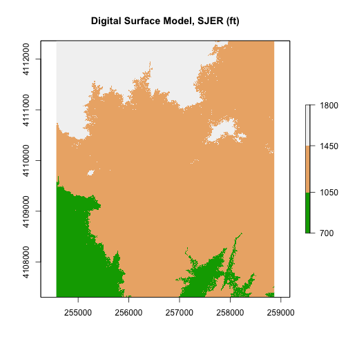
Image (RGB) Data in R

Go to our tutorial Image Raster Data in R - An Intro to learn more about working with image formatted rasters in R.

This tutorial will walk you through the fundamental principles of working with image raster data in R.

Raster Data

Raster or "gridded" data are data that are saved in pixels. In the spatial world, each pixel represents an area on the Earth's surface. An color image raster is a bit different from other rasters in that it has multiple bands. Each band represents reflectance values for a particular color or spectra of light. If the image is RGB, then the bands are in the red, green and blue portions of the electromagnetic spectrum. These colors together create what we know as a full color image.

Work with Multiple Rasters

In a previous tutorial, we loaded a single raster into R. We made sure we knew the CRS (coordinate reference system) and extent of the dataset among other key metadata attributes. This raster was a Digital Elevation Model so there was only a single raster that represented the ground elevation in each pixel. When we work with color images, there are multiple rasters to represent each band. Here we'll learn to work with multiple rasters together.

Raster Stacks

A raster stack is a collection of raster layers. Each raster layer in the raster stack needs to have the same

• projection (CRS),
• spatial extent and
• resolution.

You might use raster stacks for different reasons. For instance, you might want to group a time series of rasters representing precipitation or temperature into one R object. Or, you might want to create a color images from red, green and blue band derived rasters.

In this tutorial, we will stack three bands from a multi-band image together to create a composite RGB image.

First let's load the R packages that we need: sp and raster.

# load the raster, sp, and rgdal packages
library(raster)
library(sp)
library(rgdal)

# set the working directory to the data
#setwd("pathToDirHere")
wd <- ("~/Git/data/")
setwd(wd)

Next, let's create a raster stack with bands representing

• blue: band 19, 473.8nm
• green: band 34, 548.9nm
• red; band 58, 669.1nm

This can be done by individually assigning each file path as an object.

# import tiffs
band19 <- paste0(wd, "NEON-DS-Field-Site-Spatial-Data/SJER/RGB/band19.tif")
band34 <- paste0(wd, "NEON-DS-Field-Site-Spatial-Data/SJER/RGB/band34.tif")
band58 <- paste0(wd, "NEON-DS-Field-Site-Spatial-Data/SJER/RGB/band58.tif")

# View their attributes to check that they loaded correctly:
band19

## [1] "~/Git/data/NEON-DS-Field-Site-Spatial-Data/SJER/RGB/band19.tif"

band34

## [1] "~/Git/data/NEON-DS-Field-Site-Spatial-Data/SJER/RGB/band34.tif"

band58

## [1] "~/Git/data/NEON-DS-Field-Site-Spatial-Data/SJER/RGB/band58.tif"

Note that if we wanted to create a stack from all the files in a directory (folder) you can easily do this with the list.files() function. We would use full.names=TRUE to ensure that R will store the directory path in our list of rasters.

# create list of files to make raster stack
rasterlist1 <- list.files(paste0(wd,"NEON-DS-Field-Site-Spatial-Data/SJER/RGB", full.names=TRUE))

rasterlist1

## character(0)

Or, if your directory consists of some .tif files and other file types you don't want in your stack, you can ask R to only list those files with a .tif extension.

rasterlist2 <-  list.files(paste0(wd,"NEON-DS-Field-Site-Spatial-Data/SJER/RGB", full.names=TRUE, pattern="tif"))

rasterlist2

## character(0)

Back to creating our raster stack with three bands. We only want three of the bands in the RGB directory and not the fourth band90, so will create the stack from the bands we loaded individually. We do this with the stack() function.

# create raster stack
rgbRaster <- stack(band19,band34,band58)

# example syntax for stack from a list
#rstack1 <- stack(rasterlist1)

This has now created a stack that is three rasters thick. Let's view them.

# check attributes
rgbRaster

## class      : RasterStack 
## dimensions : 502, 477, 239454, 3  (nrow, ncol, ncell, nlayers)
## resolution : 1, 1  (x, y)
## extent     : 256521, 256998, 4112069, 4112571  (xmin, xmax, ymin, ymax)
## crs        : +proj=utm +zone=11 +datum=WGS84 +units=m +no_defs 
## names      : band19, band34, band58 
## min values :     84,    116,    123 
## max values :  13805,  15677,  14343

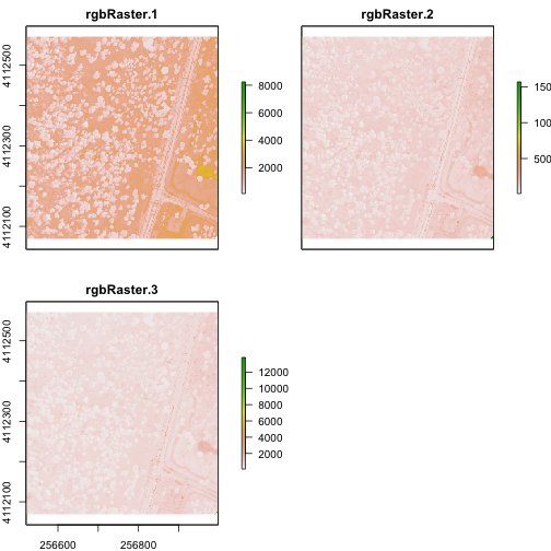
# plot stack
plot(rgbRaster)

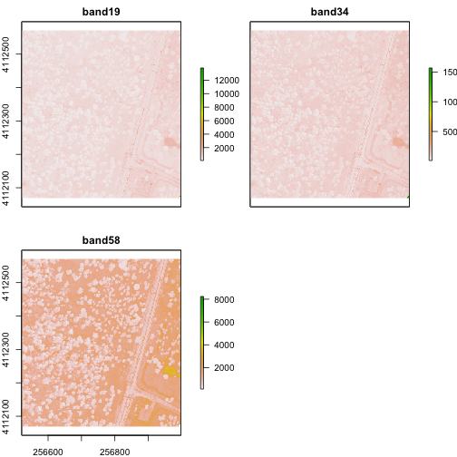
From the attributes we see the CRS, resolution, and extent of all three rasters. The we can see each raster plotted. Notice the different shading between the different bands. This is because the landscape relects in the red, green, and blue spectra differently.

Check out the scale bars. What do they represent?

This reflectance data are radiances corrected for atmospheric effects. The data are typically unitless and ranges from 0-1. NEON Airborne Observation Platform data, where these rasters come from, has a scale factor of 10,000.

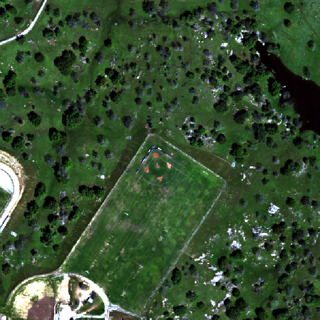
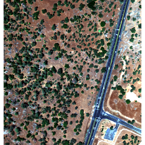
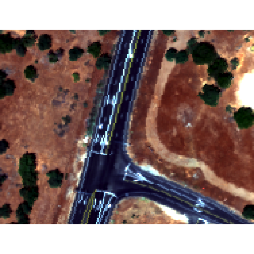
Plot an RGB Image

You can plot a composite RGB image from a raster stack. You need to specify the order of the bands when you do this. In our raster stack, band 19, which is the blue band, is first in the stack, whereas band 58, which is the red band, is last. Thus the order for a RGB image is 3,2,1 to ensure the red band is rendered first as red.

Thinking ahead to next time: If you know you want to create composite RGB images, think about the order of your rasters when you make the stack so the RGB=1,2,3.

We will plot the raster with the rgbRaster() function and the need these following arguments:

• R object to plot
• which layer of the stack is which color
• stretch: allows for increased contrast. Options are "lin" & "hist".

Let's try it.

# plot an RGB version of the stack
plotRGB(rgbRaster,r=3,g=2,b=1, stretch = "lin")

Note: read the raster package documentation for other arguments that can be added (like scale) to improve or modify the image.

Explore Raster Values - Histograms

You can also explore the data. Histograms allow us to view the distrubiton of values in the pixels.

# view histogram of reflectance values for all rasters
hist(rgbRaster)

## Warning in .hist1(raster(x, y[i]), maxpixels = maxpixels, main =
## main[y[i]], : 42% of the raster cells were used. 100000 values used.

## Warning in .hist1(raster(x, y[i]), maxpixels = maxpixels, main =
## main[y[i]], : 42% of the raster cells were used. 100000 values used.

## Warning in .hist1(raster(x, y[i]), maxpixels = maxpixels, main =
## main[y[i]], : 42% of the raster cells were used. 100000 values used.

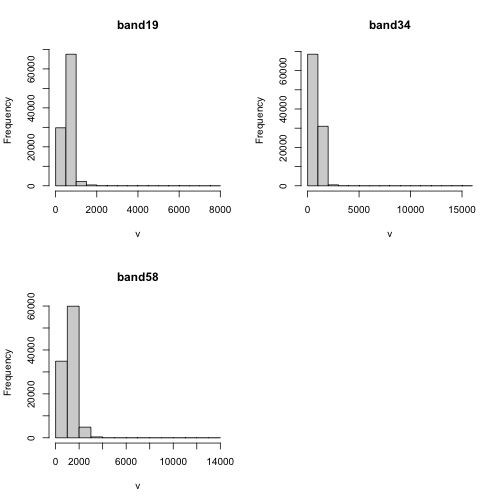
Note about the warning messages: R defaults to only showing the first 100,000 values in the histogram so if you have a large raster you may not be seeing all the values. This saves your from long waits, or crashing R, if you have large datasets.

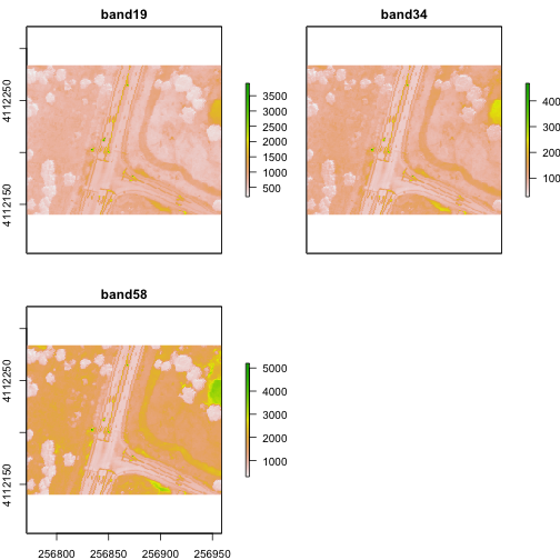
Crop Rasters

You can crop all rasters within a raster stack the same way you'd do it with a single raster.

# determine the desired extent
rgbCrop <- c(256770.7,256959,4112140,4112284)

# crop to desired extent
rgbRaster_crop <- crop(rgbRaster, rgbCrop)

# view cropped stack
plot(rgbRaster_crop)

Raster Bricks in R

In our rgbRaster object we have a list of rasters in a stack. These rasters are all the same extent, CRS and resolution. By creating a raster brick we will create one raster object that contains all of the rasters so that we can use this object to quickly create RGB images. Raster bricks are more efficient objects to use when processing larger datasets. This is because the computer doesn't have to spend energy finding the data - it is contained within the object.

# create raster brick
rgbBrick <- brick(rgbRaster)

# check attributes
rgbBrick

## class      : RasterBrick 
## dimensions : 502, 477, 239454, 3  (nrow, ncol, ncell, nlayers)
## resolution : 1, 1  (x, y)
## extent     : 256521, 256998, 4112069, 4112571  (xmin, xmax, ymin, ymax)
## crs        : +proj=utm +zone=11 +datum=WGS84 +units=m +no_defs 
## source     : memory
## names      : band19, band34, band58 
## min values :     84,    116,    123 
## max values :  13805,  15677,  14343

While the brick might seem similar to the stack (see attributes above), we can see that it's very different when we look at the size of the object.

• the brick contains all of the data stored in one object
• the stack contains links or references to the files stored on your computer

Use object.size() to see the size of an R object.

# view object size
object.size(rgbBrick)

## 5762000 bytes

object.size(rgbRaster)

## 49984 bytes

# view raster brick
plotRGB(rgbBrick,r=3,g=2,b=1, stretch = "Lin")

Notice the faster plotting? For a smaller raster like this the difference is slight, but for larger raster it can be considerable.

Write to GeoTIFF

We can write out the raster in GeoTIFF format as well. When we do this it will copy the CRS, extent and resolution information so the data will read properly into a GIS program as well. Note that this writes the raster in the order they are in. In our case, the blue (band 19) is first but most programs expect the red band first (RGB).

One way around this is to generate a new raster stack with the rasters in the proper order - red, green and blue format. Or, just always create your stacks R->G->B to start!!!

# Make a new stack in the order we want the data in 
orderRGBstack <- stack(rgbRaster$band58,rgbRaster$band34,rgbRaster$band19)

# write the geotiff
# change overwrite=TRUE to FALSE if you want to make sure you don't overwrite your files!
writeRaster(orderRGBstack,paste0(wd,"NEON-DS-Field-Site-Spatial-Data/SJER/RGB/rgbRaster.tif"),"GTiff", overwrite=TRUE)

Import A Multi-Band Image into R

You can import a multi-band image into R too. To do this, you import the file as a stack rather than a raster (which brings in just one band). Let's import the raster than we just created above.

# import multi-band raster as stack
multiRasterS <- stack(paste0(wd,"NEON-DS-Field-Site-Spatial-Data/SJER/RGB/rgbRaster.tif")) 

# import multi-band raster direct to brick
multiRasterB <- brick(paste0(wd,"NEON-DS-Field-Site-Spatial-Data/SJER/RGB/rgbRaster.tif")) 

# view raster
plot(multiRasterB)

plotRGB(multiRasterB,r=1,g=2,b=3, stretch="lin")

Want to use plot centroid values (marking the center of a plot) in x,y format to get the plot boundaries of a certain size around the centroid? This tutorial is for you!

If the plot is a circle, we can generate the plot boundary using a buffer function in R or a GIS program. However, creating a square boundary around a centroid requires an alternate approach. This tutorial presents a way to create square polygons of a given radius (referring to half of the plot's width) for each plot centroid location in a dataset.

Special thanks to jbaums from StackOverflow for helping with the SpatialPolygons code!

Our x,y coordinate centroids come in a ".csv" (Comma Separated Value) file with the plot ID that goes with the data. The data we are using today were collected at the National Ecological Observatory Network field site at the San Joaquin Experimental Range (SJER) in California.

Load .csv, Setup Plots

To work with our spatial data in R, we can use the rgdal package and the sp package. Once we've loaded these packages and set the working directory to the where our .csv file with the data is located, we can load our data.

# load the sp and rgdal packages

library(sp)
library(rgdal)

# set working directory to data folder
#setwd("pathToDirHere")
wd <- ("~/Git/data/")
setwd(wd)

# read in the NEON plot centroid data 
# `stringsAsFactors=F` ensures character strings don't import as factors
centroids <- read.csv(paste0(wd,"NEON-DS-Field-Site-Spatial-Data/SJER/PlotCentroids/SJERPlotCentroids.csv"), stringsAsFactors=FALSE)

Let's look at our data. This can be done several ways but one way is to view the structure (str()) of the data.

# view data structure
str(centroids)

## 'data.frame':	18 obs. of  5 variables:
##  $ Plot_ID : chr  "SJER1068" "SJER112" "SJER116" "SJER117" ...
##  $ Point   : chr  "center" "center" "center" "center" ...
##  $ northing: num  4111568 4111299 4110820 4108752 4110476 ...
##  $ easting : num  255852 257407 256839 256177 255968 ...
##  $ Remarks : logi  NA NA NA NA NA NA ...

We can see that our data consists of five distinct types of data:

• Plot_ID: denotes the plot
• Point: denotes where the point is taken -- all are centroids
• northing: northing coordinate for point
• easting: easting coordinate for point
• Remarks: any other remarks from those collecting the data

It would be nice to have a metadata file with this .csv to confirm the coordinate reference system (CRS) that the points are in, however, without one, based on the numbers, we can assume it is in Universal Transverse Mercator (UTM). And since we know the data are from the San Joaquin Experimental Range, that is in UTM zone 11N.

Part 1: Create Plot Boundary

Now that we understand our centroid data file, we need to set how large our plots are going to be. The next piece of code sets the "radius"" for the plots. This radius will later be used to calculate vertex locations that define the plot perimeter.

In this case, let's use a radius of 20m. This means that the edge of each plot (not the corner) is 20m from the centroid. Overall this will create a 40 m x 40 m square plot.

Units: Radius is in meters, matching the UTM CRS. If you're coordinates were in lat/long or some other CRS than you'd need to modify the code.

Plot Orientation: Our code is based on simple geometry and assumes that plots are oriented North-South. If you wanted a different orientation, adjust the math accordingly to find the corners.

# set the radius for the plots
radius <- 20 # radius in meters

# define the plot edges based upon the plot radius. 

yPlus <- centroids$northing+radius
xPlus <- centroids$easting+radius
yMinus <- centroids$northing-radius
xMinus <- centroids$easting-radius

When combining the coordinates for the vertices, it is important to close the polygon. This means that a square will have 5 instead of 4 vertices. The fifth vertex is identical to the first vertex. Thus, by repeating the first vertex coordinate (xMinus,yPlus) the polygon will be closed.

The cbind() function allows use to combine or bind together data by column. Make sure to create the vertices in an order that makes sense. We recommend starting at the NE and proceeding clockwise.

# calculate polygon coordinates for each plot centroid. 
square=cbind(xMinus,yPlus,  # NW corner
	xPlus, yPlus,  # NE corner
	xPlus,yMinus,  # SE corner
	xMinus,yMinus, # SW corner
	xMinus,yPlus)  # NW corner again - close ploygon

Next, we will associate the centroid plot ID, from the .csv file, with the plot perimeter polygon that we create below. First, we extract the Plot_ID from our data. Note that because we set stringsAsFactor to false when importing, we can extract the Plot_IDs using the code below. If we hadn't do that, our IDs would come in as factors and we'd thus have to use the code ID=as.character(centroids$Plot_ID).

# Extract the plot ID information
ID=centroids$Plot_ID

We are now left with two key "groups" of data:

• a dataframe square which has the points for our new 40x40m plots
• a listID with the Plot_IDs for each new 40x40m plot

If all we wanted to do was get these points, we'd be done. But no, we want to be able to create maps with our new plots as polygons and have them as spatial data objects for later analyses.

Part 2: Create Spatial Polygons

Now we need to convert our dataframe square into a SpatialPolygon object. This particular step is somewhat confusing. Please consider reading up on the SpatialPolygon object in R in the sp package documentation (pg 86) or check out this StackOverflow thread.

Two general consideration:

First, spatial polygons require a list of lists. Each list contains the xy coordinates of each vertex in the polygon - in order. It is always important to include the closing vertex as we discussed above -- you'll have to repeat the first vertex coordinate.

Second, we need to specify the CRS string for our new polygon. We will do this with a proj4string. We can either type in the proj4string (as we do below) or we can grab the string from another file that has CRS information. To do this, we'd use the syntax:

proj4string =CRS(as.character(FILE-NAME@crs))

For example, if we imported a GeoTIFF file called "canopy" that was in a UTM coordinate system, we could type proj4string-CRS(as.character(canopy@crs)).

Method 1: mapply function

We'll do this in two different ways. The first, using the mapply() function is far more efficient. However, the function hides a bit of what is going on so next we'll show how it is done without the function so you understand it.

# create spatial polygons from coordinates
polys <- SpatialPolygons(mapply(function(poly, id) {
	  xy <- matrix(poly, ncol=2, byrow=TRUE)
	  Polygons(list(Polygon(xy)), ID=id)
	  }, 
	split(square, row(square)), ID),
	proj4string=CRS(as.character("+proj=utm +zone=11 +datum=WGS84 +units=m +no_defs +ellps=WGS84 +towgs84=0,0,0")))

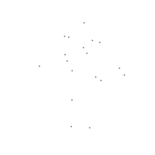
Let's create a simple plot to see our new SpatialPolygon data.

# plot the new polygons
plot(polys)

Yay! We created polygons for all of our plots!

Method 2: Using loops

Let's do the process again with simpler R code so that we understand how the process works. Keep in mind that loops are less efficient to process your data but don't hide as much under the box. Once you understand how this works, we recommend the mapply() function for your actual data processing.

# First, initialize a list that will later be populated
# a, as a placeholder, since this is temporary
a <- vector('list', length(2))

# loop through each centroid value and create a polygon
# this is where we match the ID to the new plot coordinates
for (i in 1:nrow(centroids)) {  # for each for in object centroids
	  a[[i]]<-Polygons(list(Polygon(matrix(square[i, ], ncol=2, byrow=TRUE))), ID[i]) 
	  # make it an Polygon object with the Plot_ID from object ID
	}

# convert a to SpatialPolygon and assign CRS
polysB<-SpatialPolygons(a,proj4string=CRS(as.character("+proj=utm +zone=11 +datum=WGS84 +units=m +no_defs +ellps=WGS84 +towgs84=0,0,0")))

Let's see if it worked with another simple plot.

# plot the new polygons
plot(polysB)

Good. The two methods return the same plots. We now have our new plots saved as a SpatialPolygon but how do we share that with our colleagues? One way is to turn them into shapefiles, which can be read into R, Python, QGIS, ArcGIS, and many other programs.

Part 3: Export to Shapefile

Before you can export a shapefile, you need to convert the SpatialPolygons to a SpatialPolygonDataFrame. Note that in this step you could add additional attribute data if you wanted to!

# Create SpatialPolygonDataFrame -- this step is required to output multiple polygons.
polys.df <- SpatialPolygonsDataFrame(polys, data.frame(id=ID, row.names=ID))

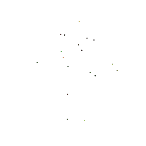
Let's check out the results before we export. And we can add color this time.

plot(polys.df, col=rainbow(50, alpha=0.5))

When we want to export a spatial object from R as a shapefile, writeOGR() is a nice function. It writes not only the shapefile, but also the associated Coordinate Reference System (CRS) information as long as it is associated with the spatial object (e.g., if it was identified when creating the SpatialPolygons object).

To do this we need the following arguments:

1. the name of the spatial object (polys.df)
2. file path from the current working directory for the directory where we want to save our shapefile. If we want it in our current directory we can simply use '.'. 3.the name of the new shapefile (2014Plots_SJER)
3. the driver which specifies the file format (ESRI Shapefile)

We can now export the spatial object as a shapefile.

# write the shapefiles 
writeOGR(polys.df, '.', '2014Plots_SJER', 'ESRI Shapefile')

And there you have it -- a shapefile with a square plot boundary around your centroids. Bring this shapefile into QGIS or whatever GIS package you prefer and have a look!

For more on working with shapefiles in R, check out our Working with Vector Data in R series .