This tutorial provides an overview of functions in the neonUtilities package in R and the neonutilities package in Python. These packages provide a toolbox of basic functionality for working with NEON data.

This tutorial is primarily an index of functions and their inputs; for more in-depth guidance in using these functions to work with NEON data, see the Download and Explore tutorial. If you are already familiar with the neonUtilities package, and need a quick reference guide to function inputs and notation, see the neonUtilities cheat sheet.

## 
## # install neonUtilities - can skip if already installed
## install.packages("neonUtilities")
## 
## # load neonUtilities
library(neonUtilities)
## 

# install neonutilities - can skip if already installed
# do this in the command line
pip install neonutilities

# load neonutilities in working environment
import neonutilities as nu

triptemp <- loadByProduct(dpID="DP1.00003.001", 
                          site=c("MOAB","ONAQ"),
                          startdate="2018-05", 
                          enddate="2018-08")

triptemp = nu.load_by_product(dpid="DP1.00003.001", 
                              site=["MOAB","ONAQ"],
                              startdate="2018-05", 
                              enddate="2018-08")

names(triptemp)

## [1] "citation_00003_RELEASE-2024" "issueLog_00003"             
## [3] "readme_00003"                "sensor_positions_00003"     
## [5] "TAAT_1min"                   "TAAT_30min"                 
## [7] "variables_00003"

temp30 <- triptemp$TAAT_30min

list2env(trip.temp, .GlobalEnv)

triptemp.keys()

## dict_keys(['TAAT_1min', 'TAAT_30min', 'citation_00003_RELEASE-2024', 'issueLog_00003', 'readme_00003', 'sensor_positions_00003', 'variables_00003'])

temp30 = triptemp["TAAT_30min"]

globals().update(triptemp)

# Modify the file path to the file location on your computer
stackByTable(filepath="~neon/data/NEON_temp-air-single.zip")

# Modify the file path to the file location on your computer
nu.stack_by_table(filepath="/neon/data/NEON_temp-air-single.zip")

SAAT30 <- readTableNEON(
  dataFile='~/stackedFiles/SAAT_30min.csv',
  varFile='~/stackedFiles/variables_00002.csv'
)

SAAT30 = nu.read_table_neon(
  dataFile='/stackedFiles/SAAT_30min.csv',
  varFile='/stackedFiles/variables_00002.csv'
)

stackByTable(filepath="~neon/data/NEON_temp-air-single.zip", 
             savepath="~data/allTemperature", saveUnzippedFiles=T)
tempsing <- stackByTable(filepath="~neon/data/NEON_temp-air-single.zip",
savepath="envt", saveUnzippedFiles=F)

nu.stack_by_table(filepath="/neon/data/NEON_temp-air-single.zip", 
                  savepath="/data/allTemperature", 
                  saveUnzippedFiles=True)
tempsing <- nu.stack_by_table(filepath="/neon/data/NEON_temp-air-single.zip",
savepath="envt",
saveUnzippedFiles=False)

zipsByProduct(dpID="DP1.00002.001", site="WREF", 
              startdate="2019-04", enddate="2019-05",
              package="basic", check.size=T)

stackByTable(filepath=paste(getwd(), 
                            "/filesToStack00002", 
                            sep=""))

nu.zips_by_product(dpid="DP1.00002.001", site="WREF", 
                   startdate="2019-04", enddate="2019-05",
                   package="basic", check_size=True)

nu.stack_by_table(filepath=os.getcwd()+
                  "/filesToStack00002")

zipsByProduct(dpID="DP1.00002.001", site="WREF", 
              startdate="2019-04", enddate="2019-05",
              package="basic", timeIndex=30, 
              check.size=T)

nu.zips_by_product(dpid="DP1.00002.001", site="WREF", 
                   startdate="2019-04", 
                   enddate="2019-05", package="basic", 
                   timeindex=30, check_size=True)

byFileAOP("DP3.30015.001", site="HOPB", 
          year=2017, check.size=T)

nu.by_file_aop(dpid="DP3.30015.001", 
               site="HOPB", year=2017, 
               check_size=True)

byTileAOP(dpID="DP3.30026.001", site="SOAP", 
          year=2018, easting=c(298755,299296),
          northing=c(4101405,4101461),
          buffer=20)

nu.by_tile_aop(dpid="DP3.30026.001", 
               site="SOAP", year=2018, 
               easting=[298755,299296],
               northing=[4101405,4101461],
               buffer=20)

The instructions below will guide you through using the neonUtilities R package in Python, via the rpy2 package. rpy2 creates an R environment you can interact with from Python.

The assumption in this tutorial is that you want to work with NEON data in Python, but you want to use the handy download and merge functions provided by the neonUtilities R package to access and format the data for analysis. If you want to do your analyses in R, use one of the R-based tutorials linked below.

For more information about the neonUtilities package, and instructions for running it in R directly, see the Download and Explore tutorial and/or the neonUtilities tutorial.

Install and set up

Before starting, you will need:

1. Python 3 installed. It is probably possible to use this workflow in Python 2, but these instructions were developed and tested using 3.7.4.
2. R installed. You don't need to have ever used it directly. We wrote this tutorial using R 4.1.1, but most other recent versions should also work.
3. rpy2 installed. Run the line below from the command line, it won't run within a Python script. See Python documentation for more information on how to install packages. rpy2 often has install problems on Windows, see "Windows Users" section below if you are running Windows.
4. You may need to install pip before installing rpy2, if you don't have it installed already.

From the command line, run pip install rpy2

Windows users

The rpy2 package was built for Mac, and doesn't always work smoothly on Windows. If you have trouble with the install, try these steps.

1. Add C:\Program Files\R\R-3.3.1\bin\x64 to the Windows Environment Variable “Path”
2. Install rpy2 manually from https://www.lfd.uci.edu/~gohlke/pythonlibs/#rpy2
   1. Pick the correct version. At the download page the portion of the files with cp## relate to the Python version. e.g., rpy2 2.9.2 cp36 cp36m win_amd64.whl is the correct download when 2.9.2 is the latest version of rpy2 and you are running Python 36 and 64 bit Windows (amd64).
   2. Save the whl file, navigate to it in windows then run pip directly on the file as follows “pip install rpy2 2.9.2 cp36 cp36m win_amd64.whl”
3. Add an R_HOME Windows environment variable with the path C:\Program Files\R\R-3.4.3 (or whichever version you are running)
4. Add an R_USER Windows environment variable with the path C:\Users\yourUserName\AppData\Local\Continuum\Anaconda3\Lib\site-packages\rpy2

Additional troubleshooting

If you're still having trouble getting R to communicate with Python, you can try pointing Python directly to your R installation path.

1. Run R.home() in R.
2. Run import os in Python.
3. Run os.environ['R_HOME'] = '/Library/Frameworks/R.framework/Resources' in Python, substituting the file path you found in step 1.

Load packages

Now open up your Python interface of choice (Jupyter notebook, Spyder, etc) and import rpy2 into your session.

import rpy2
import rpy2.robjects as robjects
from rpy2.robjects.packages import importr

Load the base R functionality, using the rpy2 function importr().

base = importr('base')
utils = importr('utils')
stats = importr('stats')

The basic syntax for running R code via rpy2 is package.function(inputs), where package is the R package in use, function is the name of the function within the R package, and inputs are the inputs to the function. In other words, it's very similar to running code in R as package::function(inputs). For example:

stats.rnorm(6, 0, 1)

FloatVector with 6 elements.

<td>
0.920298
</td>

<td>
-0.318376
</td>

<td>
0.906473
</td>

<td>
-1.004184
</td>

<td>
-0.267872
</td>

<td>
-0.470278
</td>

Suppress R warnings. This step can be skipped, but will result in messages getting passed through from R that Python will interpret as warnings.

from rpy2.rinterface_lib.callbacks import logger as rpy2_logger
import logging
rpy2_logger.setLevel(logging.ERROR)

Install the neonUtilities R package. Here I've specified the RStudio CRAN mirror as the source, but you can use a different one if you prefer.

You only need to do this step once to use the package, but we update the neonUtilities package every few months, so reinstalling periodically is recommended.

This installation step carries out the same steps in the same places on your hard drive that it would if run in R directly, so if you use R regularly and have already installed neonUtilities on your machine, you can skip this step. And be aware, this also means if you install other packages, or new versions of packages, via rpy2, they'll be updated the next time you use R, too.

The semicolon at the end of the line (here, and in some other function calls below) can be omitted. It suppresses a note indicating the output of the function is null. The output is null because these functions download or modify files on your local drive, but none of the data are read into the Python or R environments.

utils.install_packages('neonUtilities', repos='https://cran.rstudio.com/');

The downloaded binary packages are in
	/var/folders/_k/gbjn452j1h3fk7880d5ppkx1_9xf6m/T//Rtmpl5OpMA/downloaded_packages

Now load the neonUtilities package. This does need to be run every time you use the code; if you're familiar with R, importr() is roughly equivalent to the library() function in R.

neonUtilities = importr('neonUtilities')

Join data files: stackByTable()

The function stackByTable() in neonUtilities merges the monthly, site-level files the NEON Data Portal provides. Start by downloading the dataset you're interested in from the Portal. Here, we'll assume you've downloaded IR Biological Temperature. It will download as a single zip file named NEON_temp-bio.zip. Note the file path it's saved to and proceed.

Run the stackByTable() function to stack the data. It requires only one input, the path to the zip file you downloaded from the NEON Data Portal. Modify the file path in the code below to match the path on your machine.

For additional, optional inputs to stackByTable(), see the R tutorial for neonUtilities.

neonUtilities.stackByTable(filepath='/Users/Shared/NEON_temp-bio.zip');

Stacking operation across a single core.
Stacking table IRBT_1_minute
Stacking table IRBT_30_minute
Merged the most recent publication of sensor position files for each site and saved to /stackedFiles
Copied the most recent publication of variable definition file to /stackedFiles
Finished: Stacked 2 data tables and 3 metadata tables!
Stacking took 2.019079 secs
All unzipped monthly data folders have been removed.

Check the folder containing the original zip file from the Data Portal; you should now have a subfolder containing the unzipped and stacked files called stackedFiles. To import these data to Python, skip ahead to the "Read downloaded and stacked files into Python" section; to learn how to use neonUtilities to download data, proceed to the next section.

Download files to be stacked: zipsByProduct()

The function zipsByProduct() uses the NEON API to programmatically download data files for a given product. The files downloaded by zipsByProduct() can then be fed into stackByTable().

Run the downloader with these inputs: a data product ID (DPID), a set of 4-letter site IDs (or "all" for all sites), a download package (either basic or expanded), the filepath to download the data to, and an indicator to check the size of your download before proceeding or not (TRUE/FALSE).

The DPID is the data product identifier, and can be found in the data product box on the NEON Explore Data page. Here we'll download Breeding landbird point counts, DP1.10003.001.

There are two differences relative to running zipsByProduct() in R directly:

1. check.size becomes check_size, because dots have programmatic meaning in Python
2. TRUE (or T) becomes 'TRUE' because the values TRUE and FALSE don't have special meaning in Python the way they do in R, so it interprets them as variables if they're unquoted.

check_size='TRUE' does not work correctly in the Python environment. In R, it estimates the size of the download and asks you to confirm before proceeding, and the interactive question and answer don't work correctly outside R. Set check_size='FALSE' to avoid this problem, but be thoughtful about the size of your query since it will proceed to download without checking.

neonUtilities.zipsByProduct(dpID='DP1.10003.001', 
                            site=base.c('HARV','BART'), 
                            savepath='/Users/Shared',
                            package='basic', 
                            check_size='FALSE');

Finding available files
  |======================================================================| 100%

Downloading files totaling approximately 4.217543 MB
Downloading 18 files
  |======================================================================| 100%
18 files successfully downloaded to /Users/Shared/filesToStack10003

The message output by zipsByProduct() indicates the file path where the files have been downloaded.

Now take that file path and pass it to stackByTable().

neonUtilities.stackByTable(filepath='/Users/Shared/filesToStack10003');

Unpacking zip files using 1 cores.
Stacking operation across a single core.
Stacking table brd_countdata
Stacking table brd_perpoint
Copied the most recent publication of validation file to /stackedFiles
Copied the most recent publication of categoricalCodes file to /stackedFiles
Copied the most recent publication of variable definition file to /stackedFiles
Finished: Stacked 2 data tables and 4 metadata tables!
Stacking took 0.4586661 secs
All unzipped monthly data folders have been removed.

Read downloaded and stacked files into Python

We've downloaded biological temperature and bird data, and merged the site by month files. Now let's read those data into Python so you can proceed with analyses.

First let's take a look at what's in the output folders.

import os
os.listdir('/Users/Shared/filesToStack10003/stackedFiles/')

['categoricalCodes_10003.csv',
 'issueLog_10003.csv',
 'brd_countdata.csv',
 'brd_perpoint.csv',
 'readme_10003.txt',
 'variables_10003.csv',
 'validation_10003.csv']

os.listdir('/Users/Shared/NEON_temp-bio/stackedFiles/')

['IRBT_1_minute.csv',
 'sensor_positions_00005.csv',
 'issueLog_00005.csv',
 'IRBT_30_minute.csv',
 'variables_00005.csv',
 'readme_00005.txt']

Each data product folder contains a set of data files and metadata files. Here, we'll read in the data files and take a look at the contents; for more details about the contents of NEON data files and how to interpret them, see the Download and Explore tutorial.

There are a variety of modules and methods for reading tabular data into Python; here we'll use the pandas module, but feel free to use your own preferred method.

First, let's read in the two data tables in the bird data: brd_countdata and brd_perpoint.

import pandas
brd_perpoint = pandas.read_csv('/Users/Shared/filesToStack10003/stackedFiles/brd_perpoint.csv')
brd_countdata = pandas.read_csv('/Users/Shared/filesToStack10003/stackedFiles/brd_countdata.csv')

And take a look at the contents of each file. For descriptions and unit of each column, see the variables_10003 file.

brd_perpoint

brd_countdata

And now let's do the same with the 30-minute data table for biological temperature.

IRBT30 = pandas.read_csv('/Users/Shared/NEON_temp-bio/stackedFiles/IRBT_30_minute.csv')
IRBT30

Download remote sensing files: byFileAOP()

The function byFileAOP() uses the NEON API to programmatically download data files for remote sensing (AOP) data products. These files cannot be stacked by stackByTable() because they are not tabular data. The function simply creates a folder in your working directory and writes the files there. It preserves the folder structure for the subproducts.

The inputs to byFileAOP() are a data product ID, a site, a year, a filepath to save to, and an indicator to check the size of the download before proceeding, or not. As above, set check_size="FALSE" when working in Python. Be especially cautious about download size when downloading AOP data, since the files are very large.

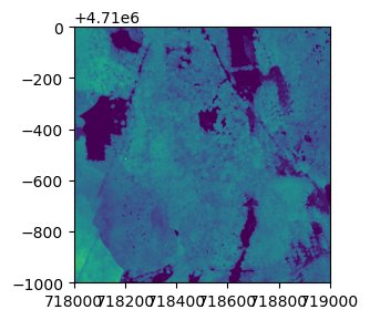
Here, we'll download Ecosystem structure (Canopy Height Model) data from Hopbrook (HOPB) in 2017.

neonUtilities.byFileAOP(dpID='DP3.30015.001', site='HOPB',
                        year='2017', check_size='FALSE',
                       savepath='/Users/Shared');

Downloading files totaling approximately 147.930656 MB 
Downloading 217 files
  |======================================================================| 100%
Successfully downloaded 217 files to /Users/Shared/DP3.30015.001

Let's read one tile of data into Python and view it. We'll use the rasterio and matplotlib modules here, but as with tabular data, there are other options available.

import rasterio
CHMtile = rasterio.open('/Users/Shared/DP3.30015.001/neon-aop-products/2017/FullSite/D01/2017_HOPB_2/L3/DiscreteLidar/CanopyHeightModelGtif/NEON_D01_HOPB_DP3_718000_4709000_CHM.tif')

import matplotlib.pyplot as plt
from rasterio.plot import show
fig, ax = plt.subplots(figsize = (8,3))
show(CHMtile)

<AxesSubplot:>

fig