Tutorial
Introduction to HDF5 Files in R
Last Updated: Apr 2, 2026
Learning Objectives
After completing this tutorial, you will be able to:
- Understand how HDF5 files can be created and structured in R using the rhdf5 libraries.
- Understand the three key HDF5 elements: the HDF5 file itself, groups, and datasets.
- Understand how to add and read attributes from an HDF5 file.
Things You’ll Need To Complete This Tutorial
To complete this tutorial you will need the most current version of R and, preferably, RStudio loaded on your computer.
R Libraries to Install:
- rhdf5: The rhdf5 package is hosted on Bioconductor not CRAN. Directions for installation are in the first code chunk.
More on Packages in R – Adapted from Software Carpentry.
Data to Download
We will use the file below in the optional challenge activity at the end of this tutorial.
NEON Teaching Data Subset: Field Site Spatial Data
These remote sensing data files provide information on the vegetation at the National Ecological Observatory Network's San Joaquin Experimental Range and Soaproot Saddle field sites. The entire dataset can be accessed by request from the NEON Data Portal.
Download DatasetSet Working Directory: This lesson assumes that you have set your working directory to the location of the downloaded and unzipped data subsets.
An overview of setting the working directory in R can be found here.
R Script & Challenge Code: NEON data lessons often contain challenges that reinforce learned skills. If available, the code for challenge solutions is found in the downloadable R script of the entire lesson, available in the footer of each lesson page.
Additional Resources
Consider reviewing the documentation for the RHDF5 package.
About HDF5
The HDF5 file can store large, heterogeneous datasets that include metadata. It
also supports efficient data slicing, or extraction of particular subsets of a
dataset which means that you don't have to read large files read into the
computers memory / RAM in their entirety in order work with them.
HDF5 in R
To access HDF5 files in R, we will use the rhdf5 library which is part of
the Bioconductor
suite of R libraries. It might also be useful to install
the
free HDF5 viewer
which will allow you to explore the contents of an HDF5 file using a graphic interface.
More about working with HDFview and a hands-on activity here.
First, let's get R setup. We will use the rhdf5 library. To access HDF5 files in R, we will use the rhdf5 library which is part of the Bioconductor suite of R packages. As of May 2020 this package was not yet on CRAN.
# Install rhdf5 package (only need to run if not already installed)
#install.packages("BiocManager")
#BiocManager::install("rhdf5")

# Call the R HDF5 Library
library("rhdf5")

# set working directory to ensure R can find the file we wish to import and where
# we want to save our files
wd <- "~/Git/data/" #This will depend on your local environment
setwd(wd)
Read more about the
rhdf5 package here.
Create an HDF5 File in R
Now, let's create a basic H5 file with one group and one dataset in it.
# Create hdf5 file
h5createFile("vegData.h5")

## [1] TRUE

# create a group called aNEONSite within the H5 file
h5createGroup("vegData.h5", "aNEONSite")

## [1] TRUE

# view the structure of the h5 we've created
h5ls("vegData.h5")

##   group      name     otype dclass dim
## 0     / aNEONSite H5I_GROUP
Next, let's create some dummy data to add to our H5 file.
# create some sample, numeric data
a <- rnorm(n=40, m=1, sd=1)
someData <- matrix(a,nrow=20,ncol=2)
Write the sample data to the H5 file.
# add some sample data to the H5 file located in the aNEONSite group
# we'll call the dataset "temperature"
h5write(someData, file = "vegData.h5", name="aNEONSite/temperature")

# let's check out the H5 structure again
h5ls("vegData.h5")

##        group        name       otype dclass    dim
## 0          /   aNEONSite   H5I_GROUP
## 1 /aNEONSite temperature H5I_DATASET  FLOAT 20 x 2
View a "dump" of the entire HDF5 file. NOTE: use this command with CAUTION if you are working with larger datasets!
# we can look at everything too
# but be cautious using this command!
h5dump("vegData.h5")

## $aNEONSite
## $aNEONSite$temperature
##              [,1]       [,2]
##  [1,]  0.33155432  2.4054446
##  [2,]  1.14305151  1.3329978
##  [3,] -0.57253964  0.5915846
##  [4,]  2.82950139  0.4669748
##  [5,]  0.47549005  1.5871517
##  [6,] -0.04144519  1.9470377
##  [7,]  0.63300177  1.9532294
##  [8,] -0.08666231  0.6942748
##  [9,] -0.90739256  3.7809783
## [10,]  1.84223101  1.3364965
## [11,]  2.04727590  1.8736805
## [12,]  0.33825921  3.4941913
## [13,]  1.80738042  0.5766373
## [14,]  1.26130759  2.2307994
## [15,]  0.52882731  1.6021497
## [16,]  1.59861449  0.8514808
## [17,]  1.42037674  1.0989390
## [18,] -0.65366487  2.5783750
## [19,]  1.74865593  1.6069304
## [20,] -0.38986048 -1.9471878

# Close the file. This is good practice.
H5close()
Add Metadata (attributes)
Let's add some metadata (called attributes in HDF5 land) to our dummy temperature data. First, open up the file.
# open the file, create a class
fid <- H5Fopen("vegData.h5")
# open up the dataset to add attributes to, as a class
did <- H5Dopen(fid, "aNEONSite/temperature")

# Provide the NAME and the ATTR (what the attribute says) for the attribute.
h5writeAttribute(did, attr="Here is a description of the data",
                 name="Description")
h5writeAttribute(did, attr="Meters",
                 name="Units")
Now we can add some attributes to the file.
# let's add some attributes to the group
did2 <- H5Gopen(fid, "aNEONSite/")

h5writeAttribute(did2, attr="San Joaquin Experimental Range",
                 name="SiteName")

h5writeAttribute(did2, attr="Southern California",
                 name="Location")

# close the files, groups and the dataset when you're done writing to them!
H5Dclose(did)

H5Gclose(did2)

H5Fclose(fid)
Working with an HDF5 File in R
Now that we've created our H5 file, let's use it! First, let's have a look at the attributes of the dataset and group in the file.
# look at the attributes of the precip_data dataset
h5readAttributes(file = "vegData.h5",
                 name = "aNEONSite/temperature")

## $Description
## [1] "Here is a description of the data"
##
## $Units
## [1] "Meters"

# look at the attributes of the aNEONsite group
h5readAttributes(file = "vegData.h5",
                 name = "aNEONSite")

## $Location
## [1] "Southern California"
##
## $SiteName
## [1] "San Joaquin Experimental Range"

# let's grab some data from the H5 file
testSubset <- h5read(file = "vegData.h5",
                 name = "aNEONSite/temperature")

testSubset2 <- h5read(file = "vegData.h5",
                 name = "aNEONSite/temperature",
                 index=list(NULL,1))
H5close()
Once we've extracted data from our H5 file, we can work with it in R.
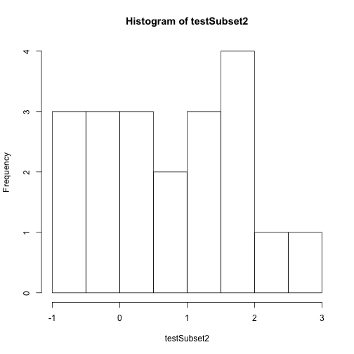
# create a quick plot of the data
hist(testSubset2)
Time to practice the skills you've learned. Open up the D17_2013_SJER_vegStr.csv in R.
- Create a new HDF5 file called
vegStructure. - Add a group in your HDF5 file called
SJER. - Add the veg structure data to that folder.
- Add some attributes the SJER group and to the data.
- Now, repeat the above with the D17_2013_SOAP_vegStr csv.
- Name your second group SOAP
Hint: read.csv() is a good way to read in .csv files.