Create A Square Buffer Around a Plot Centroid in R

Want to use plot centroid values (marking the center of a plot) in x,y format to get the plot boundaries of a certain size around the centroid? This tutorial is for you!

If the plot is a circle, we can generate the plot boundary using a buffer function in R or a GIS program. However, creating a square boundary around a centroid requires an alternate approach. This tutorial presents a way to create square polygons of a given radius (referring to half of the plot's width) for each plot centroid location in a dataset.

Special thanks to jbaums from StackOverflow for helping with the SpatialPolygons code!

Our x,y coordinate centroids come in a ".csv" (Comma Separated Value) file with the plot ID that goes with the data. The data we are using today were collected at the National Ecological Observatory Network field site at the San Joaquin Experimental Range (SJER) in California.

Load .csv, Setup Plots

To work with our spatial data in R, we can use the rgdal package and the sp package. Once we've loaded these packages and set the working directory to the where our .csv file with the data is located, we can load our data.

# load the sp and rgdal packages

library(sp)
library(rgdal)

# set working directory to data folder
#setwd("pathToDirHere")
wd <- ("~/Git/data/")
setwd(wd)

# read in the NEON plot centroid data 
# `stringsAsFactors=F` ensures character strings don't import as factors
centroids <- read.csv(paste0(wd,"NEON-DS-Field-Site-Spatial-Data/SJER/PlotCentroids/SJERPlotCentroids.csv"), stringsAsFactors=FALSE)

Let's look at our data. This can be done several ways but one way is to view the structure (str()) of the data.

# view data structure
str(centroids)

## 'data.frame':	18 obs. of  5 variables:
##  $ Plot_ID : chr  "SJER1068" "SJER112" "SJER116" "SJER117" ...
##  $ Point   : chr  "center" "center" "center" "center" ...
##  $ northing: num  4111568 4111299 4110820 4108752 4110476 ...
##  $ easting : num  255852 257407 256839 256177 255968 ...
##  $ Remarks : logi  NA NA NA NA NA NA ...

We can see that our data consists of five distinct types of data:

• Plot_ID: denotes the plot
• Point: denotes where the point is taken -- all are centroids
• northing: northing coordinate for point
• easting: easting coordinate for point
• Remarks: any other remarks from those collecting the data

It would be nice to have a metadata file with this .csv to confirm the coordinate reference system (CRS) that the points are in, however, without one, based on the numbers, we can assume it is in Universal Transverse Mercator (UTM). And since we know the data are from the San Joaquin Experimental Range, that is in UTM zone 11N.

Part 1: Create Plot Boundary

Now that we understand our centroid data file, we need to set how large our plots are going to be. The next piece of code sets the "radius"" for the plots. This radius will later be used to calculate vertex locations that define the plot perimeter.

In this case, let's use a radius of 20m. This means that the edge of each plot (not the corner) is 20m from the centroid. Overall this will create a 40 m x 40 m square plot.

Units: Radius is in meters, matching the UTM CRS. If you're coordinates were in lat/long or some other CRS than you'd need to modify the code.

Plot Orientation: Our code is based on simple geometry and assumes that plots are oriented North-South. If you wanted a different orientation, adjust the math accordingly to find the corners.

# set the radius for the plots
radius <- 20 # radius in meters

# define the plot edges based upon the plot radius. 

yPlus <- centroids$northing+radius
xPlus <- centroids$easting+radius
yMinus <- centroids$northing-radius
xMinus <- centroids$easting-radius

When combining the coordinates for the vertices, it is important to close the polygon. This means that a square will have 5 instead of 4 vertices. The fifth vertex is identical to the first vertex. Thus, by repeating the first vertex coordinate (xMinus,yPlus) the polygon will be closed.

The cbind() function allows use to combine or bind together data by column. Make sure to create the vertices in an order that makes sense. We recommend starting at the NE and proceeding clockwise.

# calculate polygon coordinates for each plot centroid. 
square=cbind(xMinus,yPlus,  # NW corner
	xPlus, yPlus,  # NE corner
	xPlus,yMinus,  # SE corner
	xMinus,yMinus, # SW corner
	xMinus,yPlus)  # NW corner again - close ploygon

Next, we will associate the centroid plot ID, from the .csv file, with the plot perimeter polygon that we create below. First, we extract the Plot_ID from our data. Note that because we set stringsAsFactor to false when importing, we can extract the Plot_IDs using the code below. If we hadn't do that, our IDs would come in as factors and we'd thus have to use the code ID=as.character(centroids$Plot_ID).

# Extract the plot ID information
ID=centroids$Plot_ID

We are now left with two key "groups" of data:

• a dataframe square which has the points for our new 40x40m plots
• a listID with the Plot_IDs for each new 40x40m plot

If all we wanted to do was get these points, we'd be done. But no, we want to be able to create maps with our new plots as polygons and have them as spatial data objects for later analyses.

Part 2: Create Spatial Polygons

Now we need to convert our dataframe square into a SpatialPolygon object. This particular step is somewhat confusing. Please consider reading up on the SpatialPolygon object in R in the sp package documentation (pg 86) or check out this StackOverflow thread.

Two general consideration:

First, spatial polygons require a list of lists. Each list contains the xy coordinates of each vertex in the polygon - in order. It is always important to include the closing vertex as we discussed above -- you'll have to repeat the first vertex coordinate.

Second, we need to specify the CRS string for our new polygon. We will do this with a proj4string. We can either type in the proj4string (as we do below) or we can grab the string from another file that has CRS information. To do this, we'd use the syntax:

proj4string =CRS(as.character(FILE-NAME@crs))

For example, if we imported a GeoTIFF file called "canopy" that was in a UTM coordinate system, we could type proj4string-CRS(as.character(canopy@crs)).

Method 1: mapply function

We'll do this in two different ways. The first, using the mapply() function is far more efficient. However, the function hides a bit of what is going on so next we'll show how it is done without the function so you understand it.

# create spatial polygons from coordinates
polys <- SpatialPolygons(mapply(function(poly, id) {
	  xy <- matrix(poly, ncol=2, byrow=TRUE)
	  Polygons(list(Polygon(xy)), ID=id)
	  }, 
	split(square, row(square)), ID),
	proj4string=CRS(as.character("+proj=utm +zone=11 +datum=WGS84 +units=m +no_defs +ellps=WGS84 +towgs84=0,0,0")))

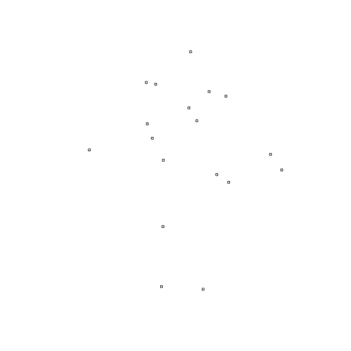
Let's create a simple plot to see our new SpatialPolygon data.

# plot the new polygons
plot(polys)

Yay! We created polygons for all of our plots!

Method 2: Using loops

Let's do the process again with simpler R code so that we understand how the process works. Keep in mind that loops are less efficient to process your data but don't hide as much under the box. Once you understand how this works, we recommend the mapply() function for your actual data processing.

# First, initialize a list that will later be populated
# a, as a placeholder, since this is temporary
a <- vector('list', length(2))

# loop through each centroid value and create a polygon
# this is where we match the ID to the new plot coordinates
for (i in 1:nrow(centroids)) {  # for each for in object centroids
	  a[[i]]<-Polygons(list(Polygon(matrix(square[i, ], ncol=2, byrow=TRUE))), ID[i]) 
	  # make it an Polygon object with the Plot_ID from object ID
	}

# convert a to SpatialPolygon and assign CRS
polysB<-SpatialPolygons(a,proj4string=CRS(as.character("+proj=utm +zone=11 +datum=WGS84 +units=m +no_defs +ellps=WGS84 +towgs84=0,0,0")))

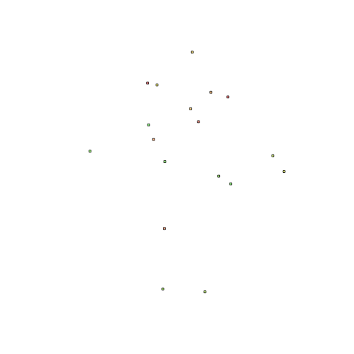
Let's see if it worked with another simple plot.

# plot the new polygons
plot(polysB)

Good. The two methods return the same plots. We now have our new plots saved as a SpatialPolygon but how do we share that with our colleagues? One way is to turn them into shapefiles, which can be read into R, Python, QGIS, ArcGIS, and many other programs.

Part 3: Export to Shapefile

Before you can export a shapefile, you need to convert the SpatialPolygons to a SpatialPolygonDataFrame. Note that in this step you could add additional attribute data if you wanted to!

# Create SpatialPolygonDataFrame -- this step is required to output multiple polygons.
polys.df <- SpatialPolygonsDataFrame(polys, data.frame(id=ID, row.names=ID))

Let's check out the results before we export. And we can add color this time.

plot(polys.df, col=rainbow(50, alpha=0.5))

When we want to export a spatial object from R as a shapefile, writeOGR() is a nice function. It writes not only the shapefile, but also the associated Coordinate Reference System (CRS) information as long as it is associated with the spatial object (e.g., if it was identified when creating the SpatialPolygons object).

To do this we need the following arguments:

1. the name of the spatial object (polys.df)
2. file path from the current working directory for the directory where we want to save our shapefile. If we want it in our current directory we can simply use '.'. 3.the name of the new shapefile (2014Plots_SJER)
3. the driver which specifies the file format (ESRI Shapefile)

We can now export the spatial object as a shapefile.

# write the shapefiles 
writeOGR(polys.df, '.', '2014Plots_SJER', 'ESRI Shapefile')

And there you have it -- a shapefile with a square plot boundary around your centroids. Bring this shapefile into QGIS or whatever GIS package you prefer and have a look!

For more on working with shapefiles in R, check out our Working with Vector Data in R series .