Classify a Lidar Raster in Python

This tutorial covers how to read in a NEON lidar Canopy Height Model (CHM) geotiff file into a Python rasterio object, shows some basic information about the raster data, and then ends with classifying the CHM into height bins.

In this tutorial, we will work with the NEON AOP L3 LiDAR ecoysystem structure (Canopy Height Model) data product. For more information about NEON data products and the CHM product DP3.30015.001, see the Ecosystem structure data product page on NEON's Data Portal.

First, let's import the required packages and set our plot display to be in-line:

import dotenv
import os
import copy
import neonutilities as nu
import numpy as np
import rasterio as rio
from rasterio.plot import show, show_hist
import matplotlib.pyplot as plt

As of June 2026, NEON requires an API token for data downloads, to reduce bot scraping and improve user support. Tokens can be generated in NEON data portal user accounts - log in to your account or create one, and go to the API Tokens section. For best practices in storing and using tokens, follow the instructions here. Once you've set up your token as an environment variable, you can load it using the python-dotenv package as follows, optionally specifying the path to the .env file in load_dotenv().

dotenv.load_dotenv()
token = os.environ.get("NEON_TOKEN")

Next, let's download a single tile (1 km x 1 km CHM file) using nu.by_tile_aop().

nu.by_tile_aop(dpid='DP3.30015.001',
               site='TEAK',
               year='2024',
               easting=320000,
               northing=4092000,
               token=token,
               savepath=r'C:\NEON_Data') # change if desired

Provisional NEON data are not included. To download provisional data, use input parameter include_provisional=True.


Continuing will download 2 NEON data files totaling approximately 2.9 MB. Do you want to proceed? (y/n)  y


Downloading 2 NEON data files totaling approximately 2.9 MB

100%|███████████████████████████████████████| 2/2 [00:00<00:00,  2.22it/s]

# iterate over directory recursively to show path of downloaded CHM.tif file
for root, dirs, files in os.walk(r'C:\NEON_Data\DP3.30015.001'):
    for name in files:
        if name.endswith('.tif'):
            chm_tile = os.path.join(root, name)
            print(chm_tile) 

C:\NEON_Data\DP3.30015.001\neon-aop-products\2024\FullSite\D17\2024_TEAK_7\L3\DiscreteLidar\CanopyHeightModelGtif\NEON_D17_TEAK_DP3_320000_4092000_CHM.tif

Open a GeoTIFF with rasterio

Let's look at the TEAK Canopy Height Model (CHM) to start. We can open and read this in Python using the rasterio.open function:

# read the chm file to the variable chm_dataset
chm_dataset = rio.open(chm_tile)

Now we can look at a few properties of this dataset to start to get a feel for the rasterio object:

print('chm_dataset:\n',chm_dataset)
print('\nshape:\n',chm_dataset.shape)
print('\nno data value:\n',chm_dataset.nodata)
print('\nspatial extent:\n',chm_dataset.bounds)
print('\ncoordinate information (crs):\n',chm_dataset.crs)

chm_dataset:
 <open DatasetReader name='C:\NEON_Data\DP3.30015.001\neon-aop-products\2024\FullSite\D17\2024_TEAK_7\L3\DiscreteLidar\CanopyHeightModelGtif\NEON_D17_TEAK_DP3_320000_4092000_CHM.tif' mode='r'>

shape:
 (1000, 1000)

no data value:
 -9999.0

spatial extent:
 BoundingBox(left=320000.0, bottom=4092000.0, right=321000.0, top=4093000.0)

coordinate information (crs):
 PROJCS["WGS 84 / UTM zone 11N",GEOGCS["WGS 84",DATUM["World Geodetic System 1984",SPHEROID["WGS 84",6378137,298.257223563]],PRIMEM["Greenwich",0],UNIT["degree",0.0174532925199433,AUTHORITY["EPSG","9122"]]],PROJECTION["Transverse_Mercator"],PARAMETER["latitude_of_origin",0],PARAMETER["central_meridian",-117],PARAMETER["scale_factor",0.9996],PARAMETER["false_easting",500000],PARAMETER["false_northing",0],UNIT["metre",1,AUTHORITY["EPSG","9001"]],AXIS["Easting",EAST],AXIS["Northing",NORTH]]

Plot the Canopy Height Map and Histogram

We can use rasterio's built-in functions show and show_hist to plot and visualize the CHM tile. It is often useful to plot a histogram of the geotiff data in order to get a sense of the range and distribution of values.

fig, (ax1, ax2) = plt.subplots(1, 2, figsize=(12,5))
show(chm_dataset, ax=ax1);

show_hist(chm_dataset, bins=50, histtype='stepfilled',
          lw=0.0, stacked=False, alpha=0.3, ax=ax2);
ax2.set_xlabel("Canopy Height (meters)");
ax2.get_legend().remove()

plt.show();

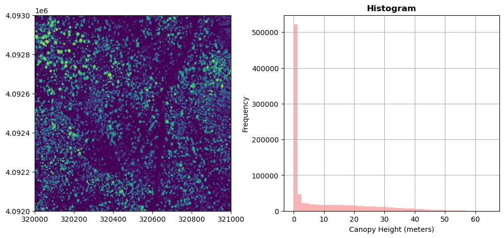
On your own, adjust the number of bins, and range of the y-axis to get a better sense of the distribution of the canopy height values. We can see that a large portion of the values are zero. These correspond to bare ground. Let's look at a histogram and plot the data without these zero values which are dominating the frequency distribution. To do this, we'll remove all values > 2 m. Due to the vertical range resolution of the lidar sensor, data collected with the older Optech Gemini sensor can only resolve the ground to within 2 m, so anything below that height would be rounded down to zero. Our newer sensors (Riegl Q780 and Optech Galaxy Prime) have a higher range resolution, so the ground can be resolved to within ~0.7 m. To see which lidar sensor collected a given site, refer to the table at the bottom of the Flight Schedules and Coverage page (https://www.neonscience.org/data-collection/flight-schedules-coverage).

chm_data = chm_dataset.read(1)
valid_data = chm_data[chm_data>2]
plt.hist(valid_data.flatten(),bins=30);

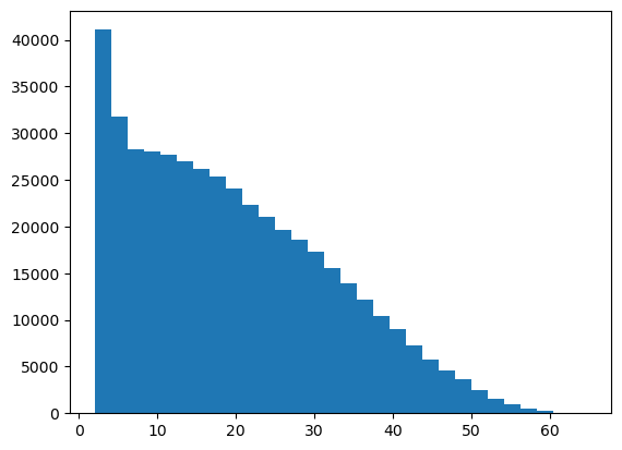
From the histogram we can see that the majority of the trees are < 60m. The frequency of tall trees rapidly drops off.

Threshold Based Raster Classification

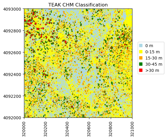
Next, we will create a classified raster object. To do this, we will use the numpy.where function to create a new raster based off boolean classifications. Let's classify the canopy height into five groups:

• Class 1: CHM = 0 m
• Class 2: 0m < CHM <= 15m
• Class 3: 10m < CHM <= 30m
• Class 4: 20m < CHM <= 45m
• Class 5: CHM > 45m

We can use np.where to find the indices where the specified criteria is met.

chm_reclass = chm_data.copy()
chm_reclass[np.where(chm_data==0)] = 1 # CHM = 0 : Class 1
chm_reclass[np.where((chm_data>0) & (chm_data<=15))] = 2 # 0m < CHM <= 10m - Class 2
chm_reclass[np.where((chm_data>15) & (chm_data<=30))] = 3 # 10m < CHM <= 20m - Class 3
chm_reclass[np.where((chm_data>30) & (chm_data<=45))] = 4 # 20m < CHM <= 30m - Class 4
chm_reclass[np.where(chm_data>45)] = 5 # CHM > 30m - Class 5

When we look at this variable, we can see that it is now populated with values between 1-5:

chm_reclass

array([[1., 1., 1., ..., 3., 3., 3.],
       [2., 2., 2., ..., 3., 3., 3.],
       [1., 2., 2., ..., 3., 3., 3.],
       ...,
       [3., 1., 4., ..., 2., 2., 2.],
       [3., 1., 1., ..., 2., 2., 2.],
       [1., 1., 1., ..., 2., 2., 1.]], shape=(1000, 1000))

Lastly we can use matplotlib to display this re-classified CHM. We will define our own colormap to plot these discrete classifications, and create a custom legend to label the classes. First, to include the spatial information in the plot, create a new variable called ext that pulls from the rasterio "bounds" field to create the extent in the expected format for plotting.

ext = [chm_dataset.bounds.left,
       chm_dataset.bounds.right,
       chm_dataset.bounds.bottom,
       chm_dataset.bounds.top]
ext

[320000.0, 321000.0, 4092000.0, 4093000.0]

import matplotlib.colors as colors
plt.figure(); 
cmap_chm = colors.ListedColormap(['lightblue','yellow','orange','green','red'])
plt.imshow(chm_reclass,extent=ext,cmap=cmap_chm)
plt.title('TEAK CHM Classification')
ax=plt.gca(); ax.ticklabel_format(useOffset=False, style='plain') #do not use scientific notation 
rotatexlabels = plt.setp(ax.get_xticklabels(),rotation=90) #rotate x tick labels 90 degrees

# Create custom legend to label the four canopy height classes:
import matplotlib.patches as mpatches
class1 = mpatches.Patch(color='lightblue', label='0 m')
class2 = mpatches.Patch(color='yellow', label='0-15 m')
class3 = mpatches.Patch(color='orange', label='15-30 m')
class4 = mpatches.Patch(color='green', label='30-45 m')
class5 = mpatches.Patch(color='red', label='>30 m')

ax.legend(handles=[class1,class2,class3,class4,class5],
          handlelength=0.7,bbox_to_anchor=(1.05, 0.4),loc='lower left',borderaxespad=0.);