Tutorial
Calculate NDVI & Extract Spectra Using Masks in Python
Last Updated: Jun 30, 2026
In this tutorial, we will calculate the Normalized Difference Vegetation Index (NDVI) using Python functions.
This tutorial works with the Level 3 Spectrometer orthorectified surface directional reflectance - mosaic data product.
Learning Objectives
After completing this tutorial, you will be able to:
- Calculate NDVI from hyperspectral data in Python.
- Calculate the mean spectra of all pixels whose NDVI is greater than or less than a specified value.
Things You’ll Need To Complete This Tutorial
To complete this tutorial, you will need:
- Python version 3.9 or higher
- Create a NEON user account
- Generate an API token for downloading data
Install Python Packages
- gdal
- h5py
- neonutilities
- pandas
- python-dotenv
- requests
Calculate NDVI & Extract Spectra with Masks
Background:
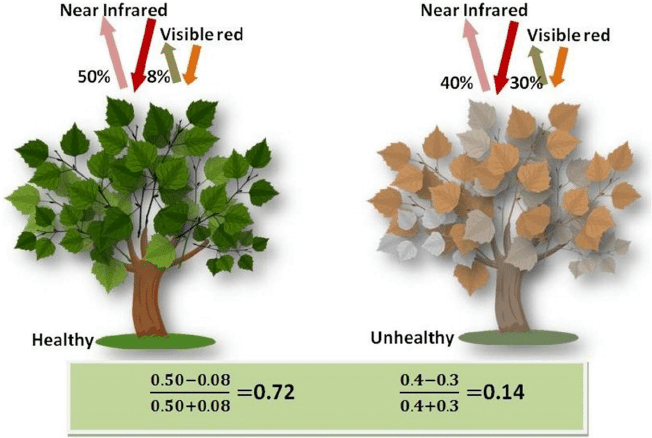
The Normalized Difference Vegetation Index (NDVI) is a standard band-ratio calculation frequently used to analyze ecological remote sensing data. NDVI indicates whether the remotely-sensed target contains live green vegetation. When sunlight strikes objects, certain wavelengths of the electromagnetic spectrum are absorbed and other wavelengths are reflected. The pigment chlorophyll in plant leaves strongly absorbs visible light (with wavelengths in the range of 400-700 nm) for use in photosynthesis. The cell structure of the leaves, however, strongly reflects near-infrared light (wavelengths ranging from 700 - 1100 nm). Plants reflect up to 60% more light in the near infrared portion of the spectrum than they do in the green portion of the spectrum. By calculating the ratio of Near Infrared (NIR) to Visible (VIS) bands in hyperspectral data, we can obtain a metric of vegetation density and health.
The formula for NDVI is: $$NDVI = \frac{(NIR - VIS)}{(NIR+ VIS)}$$
Start by setting plot preferences and loading the neon_aop_hyperspectral.py module:
import dotenv
import os, sys
from copy import copy
import requests
import neonutilities as nu
import numpy as np
import pandas as pd
import matplotlib.pyplot as plt
This next function provides a handy way to download the Python module that we will use in this lesson.
# function to download data stored on the internet in a public url to a local file
def download_url(url,download_dir):
    if not os.path.isdir(download_dir):
        os.makedirs(download_dir)
    filename = url.split('/')[-1]
    r = requests.get(url, allow_redirects=True)
    file_object = open(os.path.join(download_dir,filename),'wb')
    file_object.write(r.content)
Download the module from its location on GitHub, add the python_modules to the path and import the neon_aop_hyperspectral.py module as neon_hs.
# download the neon_aop_hyperspectral.py module from GitHub
module_url = "https://raw.githubusercontent.com/NEONScience/NEON-Data-Skills/main/tutorials/Python/AOP/aop_python_modules/neon_aop_hyperspectral.py"
download_url(module_url,'../python_modules')

# add the python_modules to the path and import the python neon download and hyperspectral functions
sys.path.insert(0, '../python_modules')

# import the neon_aop_hyperspectral module
import neon_aop_hyperspectral as neon_hs;
As of June 2026, NEON requires an API token for data downloads, to reduce bot scraping and improve user support. Tokens can be generated in NEON data portal user accounts - log in to your account or create one, and go to the API Tokens section. For best practices in storing and using tokens, follow the instructions here. Once you've set up your token as an environment variable, you can load it using the dotenv package as follows, optionally specifying the path to the .env file. Adjust the savepath variable to point to your desired location; we recommend keeping this close to the root directory since the download path to the data file will be nested.
dotenv.load_dotenv()
token = os.environ.get("NEON_TOKEN")
nu.by_tile_aop('DP3.30006.002',
               'SERC',
               2025,
               easting=368000,
               northing=4306000,
               token=token,
               include_provisional=True,
               savepath='C:/Data')
Provisional NEON data are included. To exclude provisional data, use input parameter include_provisional=False.


Continuing will download 2 NEON data files totaling approximately 661.3 MB. Do you want to proceed? (y/n)  y


Downloading 2 NEON data files totaling approximately 661.3 MB

100%|█████████████████████████████████████████████████████████████████████████████████████████████████████████████| 2/2 [01:20<00:00, 40.26s/it]
Click y when prompted to download the h5 data. Once the progress bar shows 100%, the reflectance data tile will be downloaded to the 'C:/NEON_Data/DP3.30006.002' directory. You can use the code cell below to walk through all the directories and display where the .h5 file was downloaded.
# display .h5 data in the savepath
for root, dirs, files in os.walk(r'C:\Data\DP3.30006.002'):
    for file in files:
        if file.endswith(".h5"):
             h5_tile = os.path.join(root, file)
             print(h5_tile)
C:\Data\DP3.30006.002\neon-aop-provisional-products\2025\FullSite\D02\2025_SERC_7\L3\Spectrometer\Reflectance\NEON_D02_SERC_DP3_368000_4306000_bidirectional_reflectance.h5
Read in SERC Reflectance Tile
# read the h5 reflectance file (including the full path) to the variable h5_file_name
print(f'h5_tile: {h5_tile}')
h5_tile: C:\Data\DP3.30006.002\neon-aop-provisional-products\2025\FullSite\D02\2025_SERC_7\L3\Spectrometer\Reflectance\NEON_D02_SERC_DP3_368000_4306000_bidirectional_reflectance.h5
serc_refl, serc_refl_md, wavelengths = neon_hs.aop_h5refl2array(h5_tile,'Reflectance')
Reading in C:\Data\DP3.30006.002\neon-aop-provisional-products\2025\FullSite\D02\2025_SERC_7\L3\Spectrometer\Reflectance\NEON_D02_SERC_DP3_368000_4306000_bidirectional_reflectance.h5
Extract Visible and Near Infrared Bands
Now that we have uploaded all the required functions, we can calculate NDVI and plot it. Below we print the center wavelengths of the visible band (57) and near-infrared band (89):
print('band 58 center wavelength (nm): ', wavelengths[57])
print('band 90 center wavelength (nm) : ', wavelengths[89])
band 58 center wavelength (nm):  667.457214
band 90 center wavelength (nm) :  827.793396
Calculate NDVI and Plot NDVI Maps
Here we see that band 58 represents red visible light, while band 90 is in the NIR portion of the spectrum. Let's extract these two bands from the reflectance array and calculate the ratio using the numpy.true_divide which divides arrays element-wise. This also handles a case where the denominator = 0, which would otherwise throw a warning or error.
vis = serc_refl[:,:,57]
nir = serc_refl[:,:,89]

# handle a divide by zero by setting the numpy errstate as follows
with np.errstate(divide='ignore', invalid='ignore'):
    ndvi = np.true_divide((nir-vis),(nir+vis))
    ndvi[ndvi == np.inf] = 0
    ndvi = np.nan_to_num(ndvi)
Let's take a look at the min, mean, and max values of NDVI that we calculated:
print(f'NDVI Min: {round(ndvi.min(),2)}')
print(f'NDVI Mean: {round(ndvi.mean(),2)}')
print(f'NDVI Max: {ndvi.max()}')
NDVI Min: -0.93
NDVI Mean: 0.62
NDVI Max: 1.0
We can use the function plot_aop_refl to plot this, and choose the seismic color pallette to highlight the difference between positive and negative NDVI values. Since this is a normalized index, the values should range from -1 to +1.
neon_hs.plot_aop_refl(ndvi,serc_refl_md['extent'],
                      colorlimit = (np.min(ndvi),np.max(ndvi)),
                      title='SERC Subset NDVI \n (VIS = Band 58, NIR = Band 90)',
                      cmap_title='NDVI',
                      colormap='seismic')
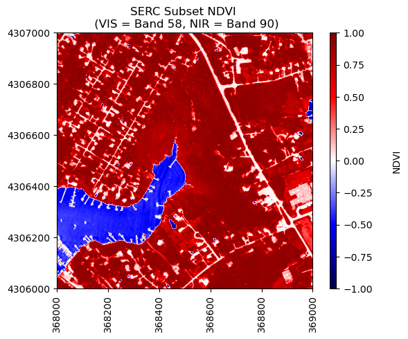
You can see that the water bodies have negative NDVI values, roads and buildings have NDVI values around 0, and vegetation has NDVI > 0. On your own, try out different color maps to see more nuances within the positive NDVI values.
Extract Spectra Using Masks
In the second part of this tutorial, we will learn how to extract the average spectra of pixels whose NDVI exceeds a specified threshold value. There are several ways to do this using numpy, including the mask functions numpy.ma, as well as numpy.where and finally using boolean indexing.
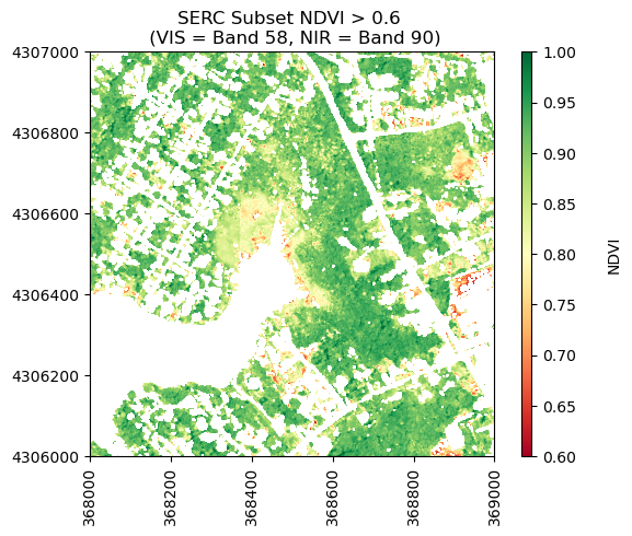
To start, lets copy the NDVI calculated above and use booleans to create an array only containing NDVI > 0.6.
# make a copy of ndvi
ndvi_gtpt6 = ndvi.copy()
#set all pixels with NDVI < 0.6 to nan, keeping only values > 0.6
ndvi_gtpt6[ndvi<0.6] = np.nan
print('Mean NDVI > 0.6:',round(np.nanmean(ndvi_gtpt6),2))
Mean NDVI > 0.6: 0.85
Now let's plot the values of NDVI after masking out values < 0.6.
neon_hs.plot_aop_refl(ndvi_gtpt6,
                      serc_refl_md['extent'],
                      colorlimit=(0.6,1),
                      title='SERC Subset NDVI > 0.6 \n (VIS = Band 58, NIR = Band 90)',
                      cmap_title='NDVI',
                      colormap='RdYlGn')
Calculate the mean spectra, thresholded by NDVI
Below we will demonstrate how to calculate statistics on arrays where you have applied a mask numpy.ma. In this example, the function calculates the mean spectra for values that remain after masking out values by a specified threshold.
import numpy.ma as ma
def calculate_mean_masked_spectra(refl_array,ndvi,ndvi_threshold,ineq='>'):
    mean_masked_refl = np.zeros(refl_array.shape[2])
    for i in np.arange(refl_array.shape[2]):
        refl_band = refl_array[:,:,i]
        if ineq == '>':
            ndvi_mask = ma.masked_where((ndvi<=ndvi_threshold) | (np.isnan(ndvi)),ndvi)
        elif ineq == '<':
            ndvi_mask = ma.masked_where((ndvi>=ndvi_threshold) | (np.isnan(ndvi)),ndvi)
        else:
            print('ERROR: Invalid inequality. Enter < or >')
        masked_refl = ma.MaskedArray(refl_band,mask=ndvi_mask.mask)
        mean_masked_refl[i] = ma.mean(masked_refl)
    return mean_masked_refl
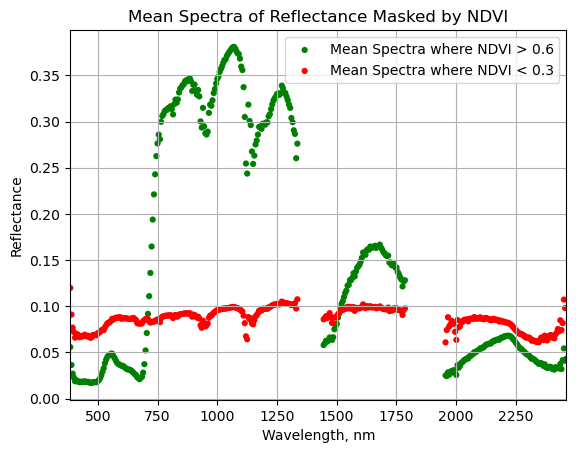
We can test out this function for various NDVI thresholds. We'll test two together, and you can try out different values on your own. Let's look at the average spectra for healthy vegetation (NDVI > 0.6), and for a lower threshold (NDVI < 0.3).
serc_ndvi_gtpt6 = calculate_mean_masked_spectra(serc_refl,ndvi,0.6)
serc_ndvi_ltpt3 = calculate_mean_masked_spectra(serc_refl,ndvi,0.3,ineq='<')
Finally, we can create a pandas dataframe of the wavelengths to plot the mean spectra.
#Remove water vapor bad band windows & last 10 bands
w = wavelengths.copy()
w[((w >= 1340) & (w <= 1445)) | ((w >= 1790) & (w <= 1955))]=np.nan
w[-10:]=np.nan;

nan_ind = np.argwhere(np.isnan(w))

serc_ndvi_gtpt6[nan_ind] = np.nan
serc_ndvi_ltpt3[nan_ind] = np.nan

#Create dataframe with masked NDVI mean spectra, scale by the reflectance scale factor
serc_ndvi_df = pd.DataFrame()
serc_ndvi_df['wavelength'] = w
serc_ndvi_df['mean_refl_ndvi_gtpt6'] = serc_ndvi_gtpt6/serc_refl_md['scale_factor']
serc_ndvi_df['mean_refl_ndvi_ltpt3'] = serc_ndvi_ltpt3/serc_refl_md['scale_factor']
Let's take a look at the first 5 values of this new dataframe:
serc_ndvi_df.head()
| wavelength | mean_refl_ndvi_gtpt6 | mean_refl_ndvi_ltpt3 | |
|---|---|---|---|
| 0 | 381.858398 | 0.005836 | 0.020809 |
| 1 | 386.868896 | 0.014392 | 0.036029 |
| 2 | 391.879395 | 0.015333 | 0.040011 |
| 3 | 396.889893 | 0.016651 | 0.045064 |
| 4 | 401.900391 | 0.012959 | 0.042483 |
Plot the masked NDVI dataframe to display the mean spectra for NDVI values that exceed 0.6 and that are less than 0.3:
ax = plt.gca();
serc_ndvi_df.plot(ax=ax,x='wavelength',y='mean_refl_ndvi_gtpt6',color='green',
                  edgecolor='none',kind='scatter',label='Mean Spectra where NDVI > 0.6',legend=True);
serc_ndvi_df.plot(ax=ax,x='wavelength',y='mean_refl_ndvi_ltpt3',color='red',
                  edgecolor='none',kind='scatter',label='Mean Spectra where NDVI < 0.3',legend=True);
ax.set_title('Mean Spectra of Reflectance Masked by NDVI')
ax.set_xlim([np.nanmin(w),np.nanmax(w)]);
ax.set_xlabel("Wavelength, nm"); ax.set_ylabel("Reflectance")
ax.grid('on');