Introduction to NEON Discrete Lidar Data in Python

pip install gdal

!pip install gdal

pip install C:\Users\username\Downloads\GDAL-3.4.3-cp39-cp39-win_amd64.whl

Overview of AOP Discrete Lidar Data Products

AOP generates several Level-1 and Level-3 (derived) data products. The Level 1 lidar data is the point cloud data, provided in laz (or zipped las) format, while the Level 3 data is provided in geotiff (.tif) raster format. Images of these two data types are shown in the figures below.

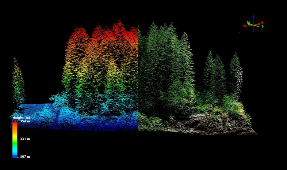Lidar Point Cloud

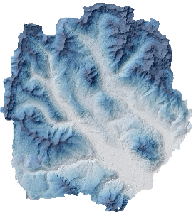Lidar Elevation Raster

The table below summarizes the NEON AOP Lidar data products. This lesson will give a brief introduction to both the Level 1 Classified Point Cloud data, as well as the Level 3 raster geotiff data products (DTM, DSM, and CHM). For more detailed information on these data products, please refer to: Airborne Remote Sensing Lidar, and/or click on the linked data product pages in the table.

The Data Product page contains important information, as well as linked Algorithm Theoretical Basis Documents (ATBDs) which provide necessary information for understanding how the data products were generated, uncertainty associated with the data, and other essential contextual information.

Lidar Point Clouds

The first part of this tutorial will be working with the Discrete Return LiDAR Point Cloud data product (DP3.30003.001) at the NEON site Guanica Forest (GUAN) in Domain 04, Puerto Rico.

Before we dig into the data, we'll need to import the required packages.

Import Packages

First, we need to import the required Python packages.

Reminder: If you haven't installed these packages (see more detailed installation instructions above), you can install them in the notebook as shown below. If the install doesn't work with a simple pip install, download the appropriate wheel file and substitute the package name with the wheel file name (including the full path). We recommend installing these packages one by one so you can make sure each package installs successfully.

!pip install requests
!pip install gdal
!pip install fiona
!pip install geopandas
!pip install rasterio
!pip install laspy
!pip install lazrs

Once all packages are successfully installed, import them as follows.

#import required packages
import os
import requests
import numpy as np
import matplotlib.pyplot as plt
import geopandas as gpd
import laspy

Now we'll pull in all the functions in the module neon_aop_download_functions.py, linked at the top of this tutorial. You can also download this file programmatically as follows:

url = "https://raw.githubusercontent.com/NEONScience/NEON-Data-Skills/main/tutorials/Python/AOP/aop_python_modules/neon_aop_download_functions.py"
response = requests.get(url)
open("neon_aop_download_functions.py", "wb").write(response.content)

First make sure this script is saved in your working directory, which we can check by navigating into that directory, or by using os.listdir. If you haven't saved it in your working directory, you will need to provide the relative path to this script when importing.

# check that script is saved in same folder:
os.listdir()

Once you've confirmed that the neon_aop_download_functions script is in your working directory, you can import the contents of this file as follows:

from neon_aop_download_functions import *

Alternatively, if you'd like to see the contents of that file in your notebook, you can use the "magic" command %load as follows:

%load neon_aop_download_functions.py

If you go this route, you will need to run the cell twice for the functions to be read into the notebook. The first run will load the functions into the cell, and the second run will load the functions into the working environment. This option of loading in the functions may be useful if you wish to modify the functions locally, eg. according to your specific workflow.

Now that we've imported in all the required packages and functions, we can get started! First let's take a look at what exactly we've imported by using the magic command %whos. Since there is no variable explorer in Jupyter Notebooks, this is a quick way to see the contents (variables, functions, modules, etc.) that have been loaded in our current environment.

%whos

Variable                      Type        Data/Info
---------------------------------------------------
download_aop_files            function    <function download_aop_fi<...>es at 0x0000029671BA80D0>
download_file                 function    <function download_file at 0x0000029671B9DF70>
download_urls                 function    <function download_urls at 0x0000029671B9DEE0>
get_file_size                 function    <function get_file_size at 0x0000029671BA8040>
gpd                           module      <module 'geopandas' from <...>\geopandas\\__init__.py'>
laspy                         module      <module 'laspy' from 'C:\<...>ges\\laspy\\__init__.py'>
list_available_urls           function    <function list_available_<...>ls at 0x000002966D323F70>
list_available_urls_by_year   function    <function list_available_<...>ar at 0x0000029671B9DE50>
np                            module      <module 'numpy' from 'C:\<...>ges\\numpy\\__init__.py'>
os                            module      <module 'os' from 'C:\\Us<...>\\Anaconda3\\lib\\os.py'>
plt                           module      <module 'matplotlib.pyplo<...>\\matplotlib\\pyplot.py'>
requests                      module      <module 'requests' from '<...>\\requests\\__init__.py'>
urllib                        module      <module 'urllib' from 'C:<...>ib\\urllib\\__init__.py'>

Data Tip

If you are unsure what a function or module does, you can find more information about the function in two ways:

1. type help(function_name), which will print out documentation below the cell, or
2. type the function name followed by ?, which will pop up the documentation at the bottom of your Jupyter Notebook window, and you can then exit out of it at your convenience

help(requests)
requests?

The functions loaded from the neon_aop_download_functions.py file also include similar documentation, so you can also use the help function with for user-defined functions, as long as the appropriate docstrings (comments) have been added.

help(list_available_urls)
list_available_urls?

Now that we've pulled in the packages needed for the first part of the tutorial, we can download a dataset from the NEON API.

First we'll start by defining variables that specify the NEON data product ID (dpID), site, and year. You can change the site code to look at a different site of your interest (for more detailed information about the NEON sites, please check out the Explore Field Sites webpage.

dpID='DP1.30003.001' 
site = 'GUAN'

We can use the function list_available_urls to see what data is available for this data product and site. This function requires two inputs: the data product ID dpID and the site ID, site.

help(list_available_urls)

Help on function list_available_urls in module neon_aop_download_functions:

list_available_urls(product, site)
    list_available urls lists the api url for a given product and site
    --------
     Inputs:
         product: the data product code (eg. 'DP3.30015.001' - CHM)
         site: the 4-digit NEON site code (eg. 'SRER', 'JORN')
    --------
    Usage:
    --------
    jorn_chm_urls = list_available_urls('DP3.30015.001','JORN')

list_available_urls(dpID,site)

['https://data.neonscience.org/api/v0/data/DP1.30003.001/GUAN/2018-05']

The AOP has only flown Puerto Rico (D04) once so far, in 2018. D04 is only on the AOP schedule every 4 years; the next campaign is scheduled for the fall of 2022, so new data is expected relatively soon!

Next let's set up some paths where we can save our downloaded data. We'll start with downloading geospatial metadata in order to get a sense of the coverage (geographic extents) of the flight area. We'll make a folder for the shapefiles (shp), kml files (which may be useful for interactively looking at the site boundaries in Google Earth), and a folder for the actual lidar (laz) data.

year='2018'
data_root_path = './data/'+site+'/'+year+'/'
shp_path = data_root_path+'shp/'
kml_path = data_root_path+'kml/'
laz_path = data_root_path+'laz/'
print(data_root_path)

./data/GUAN/2018/

Next, let's take a look at the download_aop_files function, which we'll use to download the metadata and data that we want to explore.

help(download_aop_files)

Help on function download_aop_files in module neon_aop_download_functions:

download_aop_files(product, site, year=None, download_folder='./data', match_string=None, check_size=True)
    download_aop_files downloads NEON AOP files from the AOP for a given data product, site, and 
    optional year, download folder, and 
    --------
     Inputs:
         required:
             product: the data product code (eg. 'DP3.30015.001' - CHM)
             site: the 4-digit NEON site code (eg. 'SRER', 'JORN')
         
         optional:
             year: year (eg. '2020'); default (None) is all years
             download_folder: folder to store downloaded files; default (./data) in current directory
             match_string: subset of data to match, need to use exact pattern for file name
             check_size: prompt to continue download (y/n) after displaying size; default = True
    --------
    Usage:
    --------
    download_aop_files('DP3.30015.001','JORN','2019','./data/JORN_2019/CHM','314000_3610000_CHM.tif')

The only required inputs for this function are the product and the site; optionally we can specify the year, the download_folder to save the files, and a match_string to download a subset of the data by a string. By default, the function will display the size of the files, and prompt the user to continue the download (by typing y); any other response will halt the download. This is to prevent an accidental download of a large volume of data.

Lidar Metadata

We'll start by downloading the some of the metadata, including the pdf documentation, and shape files that provide geographic information corresponding to the data. Because AOP data can be pretty large for an entire site, and you may only need to work with a subset of the data for a given site, we recommend starting with downloading only the metadata.

Lidar Documentation - QA pdfs

AOP data provides summary pdf documents, which include important information about the sensors used to collect the lidar data, acquisition parameters, processing parameters, and QA information. When working with any AOP data, we recommend reviewing this documentation, as well as referencing the relevant ATBDs.

#download the QA reports to the default download directory (./data)
download_aop_files(dpID,site,year,match_string='.pdf',check_size=False)

Download size: 11.29 MB
downloading 2018_GUAN_1_L3_discrete_lidar_processing.pdf to ./data
downloading 2018_GUAN_1_V01_LMS_QAQC.pdf to ./data

Please take a look at these pdfs on your own time!

Download and Plot Shapefile Boundaries

There are summary shape files provided along with the lidar data for each site. These summary files end with merged_tiles.shp/.shx, so we can key off that string to download only the full boundary shape file. You could also download all of the individual .shp files for each data tile (L3 data is provided in 1km x 1km tiles), by using the match string .shp, or similarly all the .kml files, if you wanted to pull the data boundaries into Google Earth and explore more interactively.

We'll download the merged_tiles shapefiles (you need to download both extensions .shp and .shx):

#download the full-boundary shape files
download_aop_files(dpID,site,year,shp_path,'merged_tiles.shp',check_size=False)
download_aop_files(dpID,site,year,shp_path,'merged_tiles.shx',check_size=False)

Download size: 0.78 kB
downloading 2018_GUAN_1_merged_tiles.shp to ./data/GUAN/2018/shp/
Download size: 0.0 kB
downloading 2018_GUAN_1_merged_tiles.shx to ./data/GUAN/2018/shp/

We can see that these files have downloaded to the expected location by listing the contents of the shp_path directory that we've made:

os.listdir(shp_path)

['2018_GUAN_1_merged_tiles.shp', '2018_GUAN_1_merged_tiles.shx']

We can see these files in the shp directory we created. Next, let's plot the boundary shapefile data using geopandas (imported as gpd) as follows:

gdf = gpd.read_file(os.path.join(shp_path,'2018_GUAN_1_merged_tiles.shp'))
gdf.plot();
ax = plt.gca(); ax.ticklabel_format(style='plain') 
ax.set_title('AOP Coverage of ' + site + ' in ' + year);
plt.xticks(rotation=90); #optionally rotate the xtick labels

GUAN 2018 Coverage

We can also pull in the boundary kml file, which can be pulled into Google Earth for a more interactive experience.

download_aop_files(dpID,site,year,kml_path,'full_boundary.kml',check_size=False) 

Download size: 0.13 kB
downloading full_boundary.kml to ./data/GUAN/2018/kml/

If you pull this into Google Earth you can see the coverage with more geographic context:

GUAN kml boundary

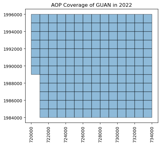
Now that we can see the extent of the tiles, we'll pick a single tile in this area to download. For this example, I'll choose the tile "724000_1985000" towards the southern part of the site, including both land and sea.

download_aop_files('DP1.30003.001',site,year,laz_path,match_string='725000_1985000_classified_point_cloud_colorized.laz')

Download size: 18.0 MB
Do you want to continue with the download? (y/n) y
downloading NEON_D04_GUAN_DP1_725000_1985000_classified_point_cloud_colorized.laz to ./data/GUAN/2018/laz/

We can use os.listdir again to check that this file successfully downloaded to the expected location. Alternatively you could go into your file explorer.

os.listdir(laz_path)

['NEON_D04_GUAN_DP1_725000_1985000_classified_point_cloud_colorized.laz']

Exploring point cloud data with laspy

Now that we've successfully downloaded a laz (or zipped las) file, we can use the laspy package to read it in! We'll do that in the next line, reading the lidar file into the variable name point_cloud:

# use os.path.join to get the full path of the laz file
laz_data_file=os.path.join(laz_path,'NEON_D04_GUAN_DP1_725000_1985000_classified_point_cloud_colorized.laz')
# read the laz file into a LasData object using laspy.read()
point_cloud=laspy.read(laz_data_file)

Reading in the file with with laspy.read() reads in both the metadata and the raw point cloud data. We can print out the point_cloud variable to show some basic information about what we've read in:

point_cloud

<LasData(1.3, point fmt: <PointFormat(3, 4 bytes of extra dims)>, 2968778 points, 2 vlrs)>

point_format.dimension_names show us the available information stored in this LasData object format:

list(point_cloud.point_format.dimension_names)

['X',
 'Y',
 'Z',
 'intensity',
 'return_number',
 'number_of_returns',
 'scan_direction_flag',
 'edge_of_flight_line',
 'classification',
 'synthetic',
 'key_point',
 'withheld',
 'scan_angle_rank',
 'user_data',
 'point_source_id',
 'gps_time',
 'red',
 'green',
 'blue',
 'reversible index (lastile)']

In the next few cells, we can explore some of these variables:

point_cloud.classification

<SubFieldView([2 2 2 ... 7 7 7])>

Let's get the set of this list to see all the unique classification values in this file. This may take a little time to run.

set(list(point_cloud.classification))

{1, 2, 5, 6, 7}

We can see that there are a several unique classification values for this site. Las files have "predefined classification schemes defined by the American Society for Photogrammetry and Remote Sensing (ASPRS)". You can refer to the ArcGIS documentation for more details.

The following table lists the LAS classification codes defined by ASPRS for these LAS versions:

Next let's take a look at what we can consider to be the main data - the geographic loation of each point in the point cloud. This can be accessed either by point_cloud.xyz. Let's take a look:

point_cloud.xyz

array([[ 7.25894810e+05,  1.98500265e+06,  2.50000000e-01],
       [ 7.25915210e+05,  1.98500018e+06,  4.20000000e-01],
       [ 7.25893550e+05,  1.98500798e+06,  2.20000000e-01],
       ...,
       [ 7.25085510e+05,  1.98583553e+06, -1.80370000e+02],
       [ 7.25101320e+05,  1.98584004e+06, -2.37230000e+02],
       [ 7.25122790e+05,  1.98583813e+06, -3.05320000e+02]])

We can see this is a 3-dimensional array, as we might expect. Let's read this into the variable xyz:

xyz = point_cloud.xyz

We can see the size (or number of points) in this array using the built-in python function len:

len(xyz)

2968778

There are > 2 million lidar points in this single 1km x 1km tile. For the rest of this exercise, we'll look at a random subset of these points, taking every100th point (you can change this subset factor, but when we visualize the data in a few steps, subsetting by a larger factor will speed up the time it takes to make the plot).

factor=100
points_dec = xyz[::factor]

These point clouds have been "colorized" by the camera RGB imagery. If you refer back to the dimension names, you can see there are a red, green, and blue attributes. We can pull these into a single array by using np.vstack:

# points = np.vstack((point_cloud.x, point_cloud.y, point_cloud.z)).transpose()
colors = np.vstack((point_cloud.red, point_cloud.green, point_cloud.blue)).transpose()

These colors have been scaled to store the color at a higher resolution, accomodated by the camera, so we'll need to re-scale the values between 0-1 in order to use them in our plot. The code below does this re-scaling, and then subsets the color data to by same factor we used to subset the xyz data.

colors_norm = (colors - np.min(colors))/np.ptp(colors)
colors_dec = colors_norm[::factor]

3D Point Cloud Visualization

Lastly, we can visualize this 3D data using matplotlib to see what the point cloud looks like.

import matplotlib.pyplot as plt
from mpl_toolkits.mplot3d import axes3d

# Plot the las data in 3D
fig = plt.figure(figsize=(6,6))
ax = fig.add_subplot(111, projection='3d')
ax.scatter(points_dec[:,0],points_dec[:,1],points_dec[:,2],color=colors_dec,s=4)
ax.set_zlim3d(-10,50)
plt.show()

GUAN colorized point cloud

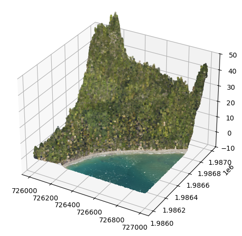
We can see a mix of both land and sea here, with slightly fewer returns on the ocean. A lot of the energy from the laser beam is absorbed in water, so it is typical to see low point density (or data gaps) over bodies of water. Remember this plot only displays 1/100th of the data, so there are many more points in the las file than are plotted here.

Lidar Raster Data - DTM, DSM, and CHM

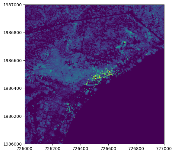
Lastly, we'll take a look at some of the derived (Level-3, or L3) data products generated from this point cloud data. NEON generates 5 different derived L3 products from the discrete data, summarized below.

In the last part of this lesson, we'll show how to read in and visualize the CHM, DTM, and DSM data using the Python package rasterio. First we'll import the package and sub-package that's used to display the data

import rasterio
from rasterio.plot import show

In the next couple cells, we'll create a path to save the raster data, and then download the L3 CHM, DTM, and DSM geotiffs of the same tile as the point cloud file we downloaded earlier. You'll see the syntax here is the same, we are just using different data product IDs and match_strings with the appropriate extensions.

l3_path = data_root_path+'L3/'

download_aop_files('DP3.30015.001',site,year,l3_path,match_string='725000_1985000_CHM.tif',check_size=False)
download_aop_files('DP3.30024.001',site,year,l3_path,match_string='725000_1985000_DTM.tif',check_size=False)
download_aop_files('DP3.30024.001',site,year,l3_path,match_string='725000_1985000_DSM.tif',check_size=False)

Next we'll read these in, using rasterio, as follows:

chm = rasterio.open(os.path.join(l3_path,'NEON_D04_GUAN_DP3_725000_1985000_CHM.tif'))
dtm = rasterio.open(os.path.join(l3_path,'NEON_D04_GUAN_DP3_725000_1985000_DTM.tif'))
dsm = rasterio.open(os.path.join(l3_path,'NEON_D04_GUAN_DP3_725000_1985000_DSM.tif'))

And finally, we can plot the data using the rasterio show function that we imported earlier.

fig, (ax1, ax2, ax3) = plt.subplots(1,3, figsize=(18,4))
show((chm), ax=ax1, title='CHM');
show((dtm), ax=ax2, title='DTM');
show((dsm), ax=ax3, title='DSM');
plt.show;

GUAN Rasters

Additional Resources

• L1 Point Clouds (.laz): If you'd like to continue exploring the point cloud data in Python using laspy, laspy website has some nice examples you can follow, now that you know how to download NEON point cloud data and read it into Python.
• L3 Rasters (.tif): Refer to the rasterio documentation for more options on plotting, and beyond in rasterio.

Python and Beyond - Other Options for working with Point Cloud Data

There are also a number of open-source tools for working with point-cloud data. Python may not be the best option for developing more rigourous processing workflows, for example. The resources below show some other recommended tools that can be integrated with Python for your analysis:

• LAStools
• PDAL (Point Data Abstraction Library)
• plas.io (free, interactive, web-based point cloud visualization)
• lidR (R package for point cloud data)