Relating Reflectance Indices to Flux Data

THIS TUTORIAL USES PRE-PREPARED DATA PROVIDED IN PERSON. CHECK BACK FOR AN UPDATED TUTORIAL INCLUDING INSTRUCTIONS FOR DATA WRANGLING.

Flux footprints represent an estimate of the region of land surface contributing to the fluxes estimated by eddy covariance. The exact footprint varies from moment to moment, due to changes in wind speed and direction, so footprints are typically presented as proportional estimates of the contribution from each point over the relevant time period. See Amiro 1998 for details and considerations about footprint calculations.

Because they represent regions of land around the flux tower, flux footprints are ideally suited to be used in combination with remotely sensed data. In this tutorial, we attempt to use flux footprints together with NDVI to estimate net ecosystem exchange (NEE), but the general principles used here can be applied to many data types in the remote sensing and eddy covariance suites (for example, canopy water content and latent heat fluxes, canopy height increment and cumulative carbon uptake, etc).

Background: NDVI in the flux footprint

Let's say we want to use reflectance data to scale up NEE, by extrapolating flux data across a larger landscape.

NEON remote sensing flights follow a detailed schedule, as described on the flight schedule page. Although flights are generally carried out at a similar time of year at each site over time, weather conditions can shift the exact date, and local weather and phenology may result in flights capturing slightly different conditions on the ground in different years. And of course, local conditions each year may result in different vegetation and soil conditions even at the same time of year and same phenological stage.

The flux footprints enable us to greatly improve the accuracy of the relationship between reflectance and fluxes - instead of guessing at the appropriate region around the tower to use for the comparison, we can use the region identified by the footprint, and weighted by the relative contribution of each pixel to the footprint.

To begin to bring together these data sources, in this tutorial, we will examine the relationship between NDVI within the flux footprint and NEE on the day(s) the remote sensing flight took place. In order to give ourselves the best odds of detecting differences, we'll focus on grasslands, where NDVI is a more reliable indicator of photosynthetic activity than, say, evergreen forests. The sites used here span a
large latitude range across the Great Plains.

Set Up Environment and Load Data

First install and load the necessary packages.

## 
## # install and load raster package
## # if raster is already installed, only the library() command
## # needs to be run
## install.packages("raster")
library(raster)
## 

Data

For this tutorial, we will need three data sets from two NEON data products: NDVI is published in Vegetation indices (DP3.30026.001), and NEE and footprints are published in Eddy covariance (DP4.00200.001). These datasets have been pre-prepared and provided on flash drives. The flux data for all sites are in one file, flux_allSites.csv. The NDVI and footprint data are in paired .grd and .gri files, one pair for each site and flight date. Finally, the flight_dates.csv file contains the date of roughly the middle of the flight campaign, to help you line up the comparable flux data with the NDVI data.

Four sites are included, three of them with data from two years. The sites, from south to north, are Konza Prairie Biological Station (KONZ), Central Plains Experimental Range (CPER), Northern Great Plains Research Laboratory (NOGP), and Dakota Coteau Field Station (DCFS).

If you're working in R, you may want to create an R Project and add the data folder to it, to keep the file paths simple. The code below assumes this structure; otherwise, you'll simply have to modify the file paths.

Start by loading the flux data and flight dates:

flux.all <- read.csv("~/data/flux_allSites.csv")
flight.dates <- read.csv("~/data/flight_dates.csv")

Let's start by viewing the data files for a single site and year, to get familiar with the data. We'll use KONZ July 2020.

Load the footprint and NDVI data. The .grd and .gri files both contain information, but loading the data only requires pointing to the .grd files.

## 
foot.KONZ <- raster("~/data/footKONZ2020-07.grd")
ndvi.KONZ <- raster("~/data/ndviKONZ2020-07.grd")
## 
## # if using Python and rasterio:
## footKONZ = rasterio.open("/data/footKONZ2020-07.grd")
## ndviKONZ = rasterio.open("/data/ndviKONZ2020-07.grd")
## 

Explore Data from One Site

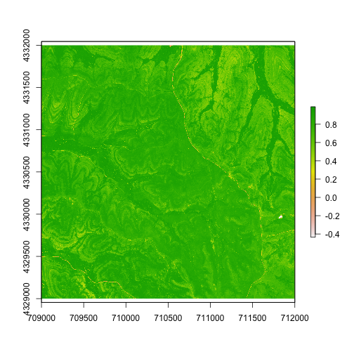
Let's start by viewing the NDVI data. The plot() function will recognize the data type and create a nice image:

plot(ndvi.KONZ)

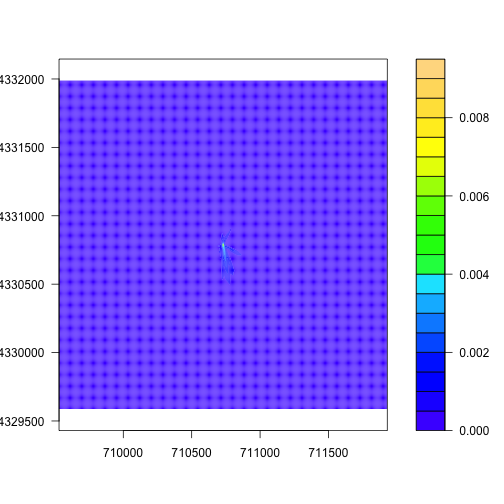
plot() also works for the flux footprints, but for these data I prefer the look of a contour plot, which shows the boundaries of different levels of influence on the flux:

filledContour(foot.KONZ, col=topo.colors(20))

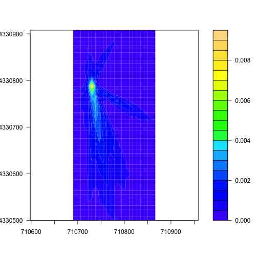
To get a better look at the region contributing the most to the flux, we can trim the raster down to pixels with a value greater than 0.0005, using the calc() and trim() functions from the raster package. First we set all pixels with a low value to zero, then trim the raster to exclude those pixels:

footAdj <- calc(foot.KONZ, 
                 fun=function(x){ x[x < 0.0005] <- 0; 
                 return(x)})
footMost <- trim(footAdj, values=0)
filledContour(footMost, col=topo.colors(20))

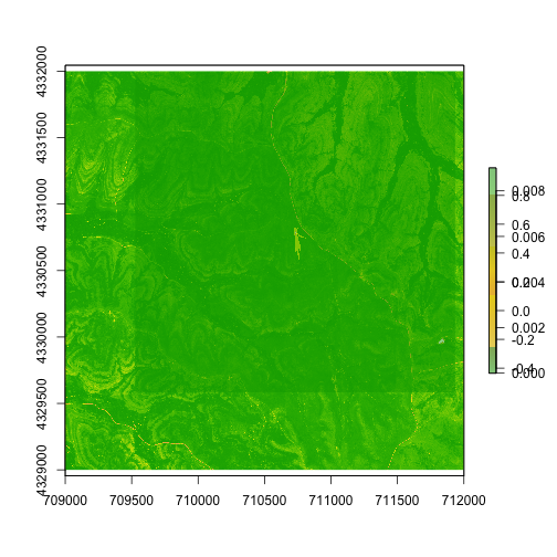
We can also overlay the NDVI and footprint data, to see where the footprint falls on the landscape. In this case we'll use the plot() function for clearer visuals:

plot(ndvi.KONZ)
plot(foot.KONZ, add=T,
     col=terrain.colors(5, alpha=0.5))

Next step: calculate mean NDVI from the sampled area, and then NDVI weighted by the contribution of the pixel to the fluxes. Starting with mean NDVI, we'll use the cellStats() function from the raster package.

cellStats(ndvi.KONZ, stat="mean", na.rm=T)

## [1] 0.7722162

To get NDVI weighted by the footprint, we need to make the two rasters comparable. Currently their boundaries don't match, and neither does their resolution. Again, the raster package has methods for this: crop() to crop the NDVI raster down to cover the same area as the footprint, and resample() to adjust the footprint raster to the resolution of the NDVI raster.

ndvi.KONZ <- crop(ndvi.KONZ, extent(foot.KONZ))
foot.KONZ <- resample(foot.KONZ, ndvi.KONZ)

In the footprint raster, each pixel's value is its proportional contribution to the flux. But now that we've resampled it to a different resolution, the sum of the pixels is no longer 1. We need to re-level the pixel values to bring them back to proportional values:

foot.KONZ <- foot.KONZ/cellStats(foot.KONZ, 
                                 stat="sum", 
                                 na.rm=T)

Now we can calculate the weighted NDVI, multiplying each NDVI pixel by its footprint weight and then using the cellStats() function as we did above:

prop.weight <- foot.KONZ*ndvi.KONZ
cellStats(prop.weight, stat="sum", 
          na.rm=T)

## [1] 0.7992741

Here we can see NDVI within the flux footprint is a little higher than NDVI across the entire region.

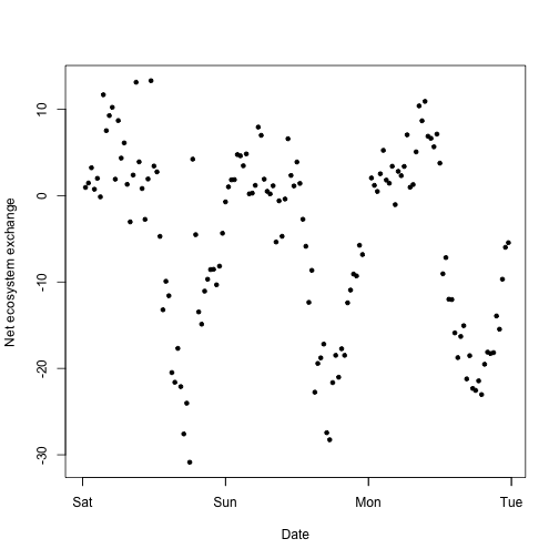
Let's take a look at the fluxes from the same time. We'll subset the flux.all table based on the site, and the dates from the flight.dates table. Let's include the date in the table, plus one on either side, since it's rare that the flights are completed in a single day (see Assumptions section below for discussion about the precise data collection dates).

flux.all$timeBgn <- as.POSIXct(flux.all$timeBgn, 
                               format="%Y-%m-%d %H:%M:%S",
                               tz="GMT")
flux.KONZ <- flux.all[which(flux.all$siteID=="KONZ" & 
                      flux.all$timeBgn>=as.POSIXct("2020-07-11", 
                                                   tz="GMT") &
                      flux.all$timeBgn<as.POSIXct("2020-07-14", 
                                                   tz="GMT")),]
plot(flux.KONZ$data.fluxCo2.nsae.flux~flux.KONZ$timeBgn, 
     pch=20, xlab="Date", ylab="Net ecosystem exchange")

Now we have fluxes and weighted NDVI from one site, but this doesn't tell us much by itself! We need context from other sites and years.

Calculate Weighted NDVI and Fluxes Across Sites

In the next two code chunks, we'll write a function to make the weighted NDVI calculations above, and then loop over the sites and dates in the dataset. I encourage you to try out writing the function and the loop yourself, especially if you're working on developing your coding skills. But if you're not familiar with how to do this, you can copy the code as written below.

Function to calculate footprint-weighted NDVI:

foot.weighted <- function(ndvi.raster, foot.raster) {

  ndvi.foot <- crop(ndvi.raster, extent(foot.raster))
  foot.ndvi <- raster::resample(foot.raster, ndvi.foot)
  foot.ndvi <- foot.ndvi/cellStats(foot.ndvi, stat="sum", na.rm=T)
  comb <- foot.ndvi*ndvi.foot
  w.ndvi <- cellStats(comb, stat="sum", na.rm=T)
  return(w.ndvi)
  
}

Loop over the rasters of all sites and dates, reading in both the NDVI and footprint rasters and applying the weighting function. If your data aren't in a project folder, or your folder structure differs, you'll need to adjust the file paths at the start of the for loop.

flight.dates$month <- substring(flight.dates$FlightDate, 1, 7)
ndvi.w <- character()
for(i in unique(flight.dates$Site)) {
  
  ffls <- list.files("~/data", "foot", full.names=T)
  afls <- list.files("~/data", "ndvi", full.names=T)
  ffls <- grep(".grd$", ffls, value=T)
  afls <- grep(".grd$", afls, value=T)

  flight.dates.i <- flight.dates[which(flight.dates$Site==i),]
  
  for(j in unique(flight.dates.i$month)) {
    
    footfl <- grep(i, ffls, value=T)
    footfl <- grep(j, footfl, value=T)
    if(length(footfl)==0) {next}
    nfl <- grep(i, afls, value=T)
    nfl <- grep(j, nfl, value=T)
    
    foot <- raster(footfl)
    ndvi <- raster(nfl)
    
    nw <- foot.weighted(ndvi, foot)
    ndvi.w <- rbind(ndvi.w, c(i, j, nw))
    
  }
  
}

ndvi.w <- data.frame(ndvi.w)
names(ndvi.w) <- c('site','month','ndvi')
ndvi.w$ndvi <- as.numeric(ndvi.w$ndvi)

ndvi.w

##   site   month      ndvi
## 1 KONZ 2019-05 0.7561873
## 2 KONZ 2020-07 0.7992741
## 3 NOGP 2019-07 0.7307495
## 4 NOGP 2021-06 0.4495142
## 5 CPER 2020-06 0.2578832
## 6 CPER 2021-06 0.3197897
## 7 DCFS 2020-06 0.7258271

Now we have a table of footprint-weighted NDVI for every site and month of data collection. Great! All we need now is flux data to compare it to.

We'll again loop over the sites and dates in the dataset, but this time we'll subset the flux dataset to the date of the flight, plus one day on either side, and calculate the daily net ecosystem exchange. Again, I encourage you to give this a try on your own, but the code I used to do it is in the next code chunk.

ndvi.w$flux <- NA
flight.dates$FlightDate <- as.POSIXct(flight.dates$FlightDate, 
                                      tz="GMT")
for(i in 1:nrow(flight.dates)) {
  
  flux.sub <- flux.all[which(flux.all$siteID==
                               flight.dates$Site[i] & 
                        flux.all$timeBgn>=
                          I(flight.dates$FlightDate[i]-86400) &
                        flux.all$timeBgn<
                          I(flight.dates$FlightDate[i]+86400)),]
  fl <- mean(flux.sub$data.fluxCo2.nsae.flux, na.rm=T)
  ndvi.w$flux[which(ndvi.w$site==flight.dates$Site[i] & 
                      ndvi.w$month==flight.dates$month[i])] <- fl
  
}

# convert to units of grams of carbon per meter squared per day
ndvi.w$flux <- ndvi.w$flux*1e-6*12.011*86400

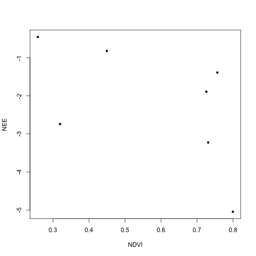
Now plot NEE against weighted NDVI:

plot(ndvi.w$flux~ndvi.w$ndvi, 
     xlab="NDVI", ylab="NEE",
     pch=20)

To get a little more insight, let's plot the site code for each data point:

plot(ndvi.w$flux~ndvi.w$ndvi, 
     xlab="NDVI", ylab="NEE",
     type="n", pch=20)
text(ndvi.w$ndvi, ndvi.w$flux,
     labels=ndvi.w$site, cex=0.5)

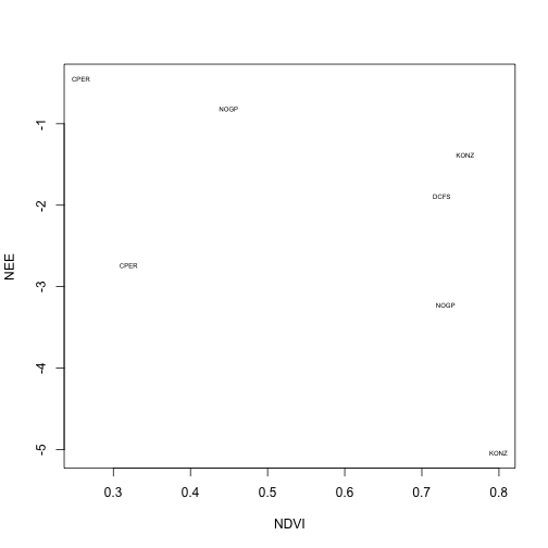
We can see that increasing NDVI is associated with increased carbon uptake. But we calculated this using overall NEE, which includes respiration. Depending on our analysis, it might be more appropriate to try to build a model to predict uptake, and to model respiration separately.

To do this properly, we'd need to use flux partitioning methods, but we can get a very crude idea of what the results might look like by re-calculating our NEE estimate using only the negative values from each day. We'll re-use the flux calculation for loop above:

ndvi.w$dayflux <- NA
for(i in 1:nrow(flight.dates)) {
  
  flux.sub <- flux.all[which(flux.all$siteID==
                               flight.dates$Site[i] & 
                        flux.all$timeBgn>=
                          I(flight.dates$FlightDate[i]-86400) &
                        flux.all$timeBgn<
                          I(flight.dates$FlightDate[i]+86400)),]
  fl <- mean(flux.sub$data.fluxCo2.nsae.flux
             [which(flux.sub$data.fluxCo2.nsae.flux<0)], na.rm=T)
  ndvi.w$dayflux[which(ndvi.w$site==flight.dates$Site[i] & 
                      ndvi.w$month==flight.dates$month[i])] <- fl
  
}

ndvi.w$dayflux <- ndvi.w$dayflux*1e-6*12.011*86400

And plot carbon uptake as above:

plot(ndvi.w$dayflux~ndvi.w$ndvi, 
     xlab="NDVI", ylab="Daytime NEE",
     type="n", pch=20)
text(ndvi.w$ndvi, ndvi.w$dayflux,
     labels=ndvi.w$site, cex=0.5)

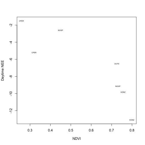
The relationship is much tighter when we consider only net uptake values.

Assumptions, Simplifications, and Further Possibilities

As mentioned, it's best to model GPP and respiration separately, and we would expect NDVI to have a much stronger relationship with GPP than respiration. But that's not the only way our analysis here is limited relative to what's possible.

To simplify our calculations of which fluxes correspond to the NDVI values, I provided the flight.dates table, which contains a single date for each site and year. In reality, the flights can span several days, which aren't always consecutive. In addition to simplifying the flight info, the flux footprints in the provided dataset are averaged over all the days when the plane was overhead.

The data product Spectrometer orthorectified surface directional reflectance - mosaic (DP3.30006.001) includes data tiles containing the flight date when each pixel was collected. The expanded package of the flux data product, Bundled data products - eddy covariance (DP4.00200.001) includes flux footprints for every half-hourly flux calculation interval. It is possible to use these datasets to calculate the contribution to the flux of every NDVI pixel at the time it was observed. However, this would be a very elaborate calculation, and before going down that road, consider the scientific question you're trying to answer. Given what you know about uncertainties in fluxes, uncertainties in NDVI, and the relative rates of change of NDVI and NEE over time, is your question sensitive to this level of detail?

Considering sensitivity raises another question: How important were the flux footprints to our analysis? How different would the results be if we simply calculated NDVI for, say, a one kilometer radius around the tower? This is an easy question to answer, with only a small modification to the code above. Give it a try, and again, consider the types of analyses that might demand different levels of precision.

Finally, note that in our dataset, we had three pairs of repeat measurements at the same site. In general, we would expect much better model predictions within a site than between sites. And we restricted ourselves to Great Plains grasslands. How would we expect this exercise to differ if we expanded into other site types?