You will need an free online Plotly account to post & share you plots online. But
you can create the plots and use them on your local computer without an account.
If you do not wish to share plots online you can skip to
Step 3: Create Plotly plot.
Note: Plotly doesn't just work with R -- other programs include Python, MATLAB,
Excel, and JavaScript.
Step 1: Create account
If you do not already have an account, you need to set up an account by visiting
the Plotly website and following
the directions there.
Step 2: Connect account to R
To share plots from R (or RStudio) to Plotly, you have to connect to your
account. This is done through an API (Application Program Interface). You can
find your username & API key in your profile settings on the Plotly website
under the "API key" menu option.
To link your account to your R, use the following commands, substituting in your
own username & key as appropriate.
# set plotly user name
Sys.setenv("plotly_username"="YOUR_USERNAME")
# set plotly API key
Sys.setenv("plotly_api_key"="YOUR_KEY")
Step 3: Create Plotly plot
There are lots of ways to plot with the plotly package. We briefly describe two
basic functions plotly() and ggplotly(). For more information on plotting in
R with Plotly, check out the
Plotly R library page.
Here we use the example dataframe economics that comes with the package.
# load packages
library(ggplot2) # to create plots and feed to ggplotly()
library(plotly)  # to create interactive plots

# view str of example dataset
str(economics)

## tibble [574 × 6] (S3: spec_tbl_df/tbl_df/tbl/data.frame)
##  $ date    : Date[1:574], format: "1967-07-01" "1967-08-01" ...
##  $ pce     : num [1:574] 507 510 516 512 517 ...
##  $ pop     : num [1:574] 198712 198911 199113 199311 199498 ...
##  $ psavert : num [1:574] 12.6 12.6 11.9 12.9 12.8 11.8 11.7 12.3 11.7 12.3 ...
##  $ uempmed : num [1:574] 4.5 4.7 4.6 4.9 4.7 4.8 5.1 4.5 4.1 4.6 ...
##  $ unemploy: num [1:574] 2944 2945 2958 3143 3066 ...

# plot with the plot_ly function
unempPerCapita <- plot_ly(x =economics$date, y = economics$unemploy/economics$pop)
To make your plotly plot in R, run the following line:
unempPerCapita
Note: This plot is interactive within the R environment but is not as posted on
this website.
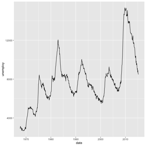
If you already use ggplot to create your plots, you can directly turn your
ggplot objects into interactive plots with ggplotly().
## plot with ggplot, then ggplotly

unemployment <- ggplot(economics, aes(date,unemploy)) + geom_line()
unemployment
To make your plotly plot in R, run the following line:
ggplotly(unemployment)
Note: This plot is interactive within the R environment but is not as posted on
this website.
Step 4: Publish to Plotly
The function plotly_POST() allows you to post any plotly plot to your account.
# publish plotly plot to your plotly online account
api_create(unemployment)
Examples
The plots below were generated using R code that harnesses the power of the
ggplot2 and the plotly packages. The plotly code utilizes the
RopenSci plotly packages - check them out!
Data Tip Are you a Python user? Use matplotlib
to create and publish visualizations.
After completing this tutorial, you will be able to:
Explain what the Hierarchical Data Format (HDF5) is.
Describe the key benefits of the HDF5 format, particularly related to big data.
Describe both the types of data that can be stored in HDF5 and how it can be stored/structured.
About Hierarchical Data Formats - HDF5
The Hierarchical Data Format version 5 (HDF5), is an open source file format
that supports large, complex, heterogeneous data. HDF5 uses a "file directory"
like structure that allows you to organize data within the file in many different
structured ways, as you might do with files on your computer. The HDF5 format
also allows for embedding of metadata making it self-describing.
**Data Tip:** HDF5 is one hierarchical data format,
that builds upon both HDF4 and NetCDF (two other hierarchical data formats).
Read more about HDF5 here.
Hierarchical Structure - A file directory within a file
The HDF5 format can be thought of as a file system contained and described
within one single file. Think about the files and folders stored on your computer.
You might have a data directory with some temperature data for multiple field
sites. These temperature data are collected every minute and summarized on an
hourly, daily and weekly basis. Within one HDF5 file, you can store a similar
set of data organized in the same way that you might organize files and folders
on your computer. However in a HDF5 file, what we call "directories" or "folders"
on our computers, are called groups and what we call files on our
computer are called datasets.
2 Important HDF5 Terms
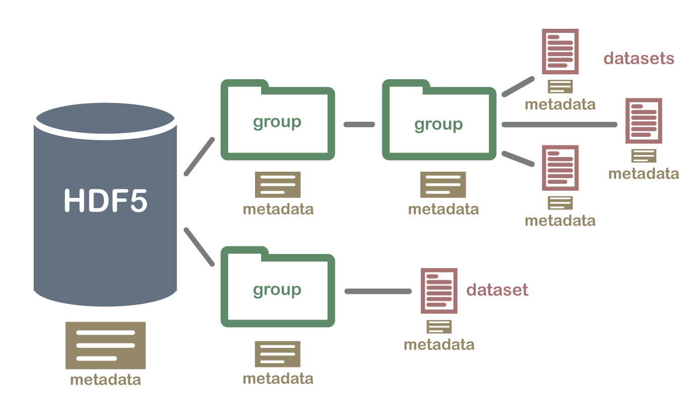
Group: A folder like element within an HDF5 file that might contain other
groups OR datasets within it.
Dataset: The actual data contained within the HDF5 file. Datasets are often
(but don't have to be) stored within groups in the file.
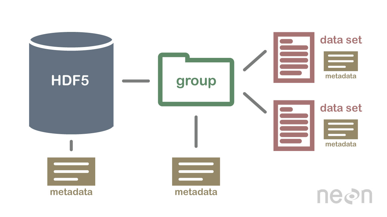
An example HDF5 file structure which contains groups, datasets and associated metadata.
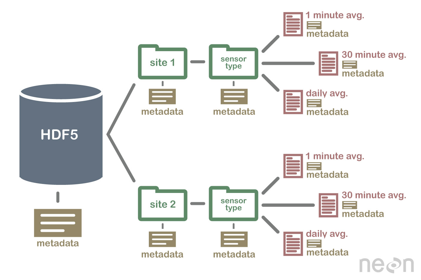
An HDF5 file containing datasets, might be structured like this:
An example HDF5 file structure containing data for multiple field sites and also containing various datasets (averaged at different time intervals).
HDF5 is a Self Describing Format
HDF5 format is self describing. This means that each file, group and dataset
can have associated metadata that describes exactly what the data are. Following
the example above, we can embed information about each site to the file, such as:
The full name and X,Y location of the site
Description of the site.
Any documentation of interest.
Similarly, we might add information about how the data in the dataset were
collected, such as descriptions of the sensor used to collect the temperature
data. We can also attach information, to each dataset within the site group,
about how the averaging was performed and over what time period data are available.
One key benefit of having metadata that are attached to each file, group and
dataset, is that this facilitates automation without the need for a separate
(and additional) metadata document. Using a programming language, like R or
Python, we can grab information from the metadata that are already associated
with the dataset, and which we might need to process the dataset.
HDF5 files are self describing - this means that all elements
(the file itself, groups and datasets) can have associated metadata that
describes the information contained within the element.
Compressed & Efficient subsetting
The HDF5 format is a compressed format. The size of all data contained within
HDF5 is optimized which makes the overall file size smaller. Even when
compressed, however, HDF5 files often contain big data and can thus still be
quite large. A powerful attribute of HDF5 is data slicing, by which a
particular subsets of a dataset can be extracted for processing. This means that
the entire dataset doesn't have to be read into memory (RAM); very helpful in
allowing us to more efficiently work with very large (gigabytes or more) datasets!
Heterogeneous Data Storage
HDF5 files can store many different types of data within in the same file. For
example, one group may contain a set of datasets to contain integer (numeric)
and text (string) data. Or, one dataset can contain heterogeneous data types
(e.g., both text and numeric data in one dataset). This means that HDF5 can store
any of the following (and more) in one file:
Temperature, precipitation and PAR (photosynthetic active radiation) data for
a site or for many sites
A set of images that cover one or more areas (each image can have specific
spatial information associated with it - all in the same file)
A multi or hyperspectral spatial dataset that contains hundreds of bands.
Field data for several sites characterizing insects, mammals, vegetation and
meteorology.
A set of images that cover one or more areas (each image can have unique
spatial information associated with it)
And much more!
Open Format
The HDF5 format is open and free to use. The supporting libraries (and a free
viewer), can be downloaded from the
HDF Group
website. As such, HDF5 is widely supported in a host of programs, including
open source programming languages like R and Python, and commercial
programming tools like Matlab and IDL. Spatial data that are stored in HDF5
format can be used in GIS and imaging programs including QGIS, ArcGIS, and
ENVI.
Summary Points - Benefits of HDF5
Self-Describing The datasets with an HDF5 file are self describing. This
allows us to efficiently extract metadata without needing an additional metadata
document.
Supporta Heterogeneous Data: Different types of datasets can be contained
within one HDF5 file.
Supports Large, Complex Data: HDF5 is a compressed format that is designed
to support large, heterogeneous, and complex datasets.
Supports Data Slicing: "Data slicing", or extracting portions of the
dataset as needed for analysis, means large files don't need to be completely
read into the computers memory or RAM.
Open Format - wide support in the many tools: Because the HDF5 format is
open, it is supported by a host of programming languages and tools, including
open source languages like R and Python and open GIS tools like QGIS.
In this tutorial, we will show how to read and extract NEON reflectance data stored within an HDF5 file using R.
Learning Objectives
After completing this tutorial, you will be able to:
Explain how HDF5 data can be used to store spatial data and the benefits of this format when working with large spatial data cubes.
Extract metadata from HDF5 files.
Slice or subset HDF5 data. You will extract one band of pixels.
Plot a matrix as an image and a raster.
Export a final GeoTIFF (spatially projected) that can be used both in further analysis and in common GIS tools like QGIS.
Things You’ll Need To Complete This Tutorial
To complete this tutorial you will need the most current version of R and, preferably, RStudio installed on your computer.
As of June 2026, NEON requires an API token for data downloads, to reduce bot scraping and improve user support. Tokens can be generated in NEON data portal user accounts - log in to your account or create one, and go to the API Tokens section. For best practices in storing and using tokens, follow the instructions here.
R Script & Challenge Code: NEON data lessons often contain challenges to reinforce skills. If available, the code for challenge solutions is found in the downloadable R script of the entire lesson, available in the footer of each lesson page.
About Hyperspectral Remote Sensing Data
The electromagnetic spectrum is composed of thousands of bands representing different types of light energy. Imaging spectrometers (instruments that collect hyperspectral data) break the electromagnetic spectrum into groups of bands that support classification of objects by their spectral properties on the Earth's surface. Hyperspectral data consists of many bands - up to hundreds of bands - that span a portion of the electromagnetic spectrum, from the visible to the Short Wave Infrared (SWIR) regions.
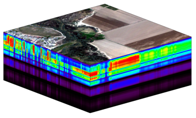
The NEON imaging spectrometer (NIS) collects data within the 380 nm to 2510 nm portions of the electromagnetic spectrum within bands that are approximately 5 nm in width. This results in a hyperspectral data cube that contains approximately 426 bands - which means BIG DATA.
A data cube of NEON hyperspectral data. Each layer in the cube represents a band.
The HDF5 data model natively compresses data stored within it (makes it smaller) and supports data slicing (extracting only the portions of the data that you need to work with rather than reading the entire dataset into memory). These features make it ideal for working with large data cubes such as those generated by imaging spectrometers, in addition to supporting spatial data and associated metadata.
In this tutorial we will demonstrate how to read and extract spatial raster data stored within an HDF5 file using R.
Read HDF5 data into R
We will use the terra and rhdf5 packages to read in the HDF5 file that contains hyperspectral data for the NEON San Joaquin (SJER) field site.
Let's start by calling the needed packages and reading in our NEON HDF5 file.
Please be sure that you have at least version 2.10 of rhdf5 installed. Use:
packageVersion("rhdf5") to check the package version.
Data Tip: To update all packages installed in R, use update.packages().
# Load `terra` and `rhdf5` packages to read NIS data into R

library(terra)

library(rhdf5)

library(neonUtilities)

# Read in NEON_TOKEN (see "Things You'll Need to Complete This Tutorial" section to set this up)

token <- Sys.getenv("NEON_TOKEN")
Set the working directory to ensure R can find the file we are importing, and we know where the file is being saved. You can move the file that is downloaded afterward, but be sure to re-set the path to the file.
data_dir <- "~/data/" #This will depend on your local environment
We can use the neonUtilities function byTileAOP to download a single reflectance tile. You can run help(byTileAOP) to see more details on what the various inputs are. For this exercise, we'll specify the UTM Easting and Northing to be (257500, 4112500), which will download the tile with the lower left corner (257000,4112000). By default, the function will check the size total size of the download and ask you whether you wish to proceed (y/n). This file is ~672.7 MB, so make sure you have enough space on your local drive. You can set check.size=FALSE if you want to download without a prompt.
byTileAOP(dpID='DP3.30006.001',

          site='SJER',

          year='2021',

          easting=257500,

          northing=4112500,

          check.size=TRUE, # set to FALSE if you don't want to enter y/n

          savepath = data_dir,

          token=token)
This file will be downloaded into a nested subdirectory under the ~/data folder, inside a folder named DP3.30006.001 (the Data Product ID). The file should show up in this location: ~/data/DP3.30006.001/neon-aop-products/2021/FullSite/D17/2021_SJER_5/L3/Spectrometer/Reflectance/NEON_D17_SJER_DP3_257000_4112000_reflectance.h5.
Data Tip: To make sure you are pointing to the correct path, look in the ~/data folder and navigate to where the .h5 file is saved, or use the R command list.files(path=data_dir,pattern="\\.h5$",recursive=TRUE,full.names=TRUE) to display the full path of the .h5 file. Note, if you have any other .h5 files downloaded in this folder, it will display all of the hdf5 files.
# Define the h5 file name to be opened

h5_file <- paste0(data_dir,"DP3.30006.001/neon-aop-products/2021/FullSite/D17/2021_SJER_5/L3/Spectrometer/Reflectance/NEON_D17_SJER_DP3_257000_4112000_reflectance.h5")
You can use h5ls and/or View(h5ls(...)) to look at the contents of the hdf5 file, as follows:
# look at the HDF5 file structure

View(h5ls(h5_file,all=T))
When you look at the structure of the data, take note of the "map info" dataset, the Coordinate_System group, and the wavelength and Reflectance datasets. The Coordinate_System folder contains the spatial attributes of the data including its EPSG Code, which is easily converted to a Coordinate Reference System (CRS). The CRS documents how the data are physically located on the Earth. The wavelength dataset contains the wavelength values for each band in the data. The Reflectance dataset contains the image data that we will use for both data processing and visualization.
About Hyperspectral Remote Sensing Data -this tutorial explains more about metadata and important concepts associated with multi-band (multi and hyperspectral) rasters.
Data Tip - HDF5 Structure: Note that the structure of individual HDF5 files may vary depending on who produced the data. In this case, the Wavelength and reflectance data within the file are both h5 datasets. However, the spatial information is contained within a group. Data downloaded from another organization (like NASA) may look different. This is why it's important to explore the data as a first step!
We can use the h5readAttributes() function to read and extract metadata from the HDF5 file. Let's start by learning about the wavelengths described within this file.
# get information about the wavelengths of this dataset

wavelengthInfo <- h5readAttributes(h5_file,"/SJER/Reflectance/Metadata/Spectral_Data/Wavelength")

wavelengthInfo

## $Description
## [1] "Central wavelength of the reflectance bands."
##
## $Units
## [1] "nanometers"
Next, we can use the h5read function to read the data contained within the HDF5 file. Let's read in the wavelengths of the band centers:
# read in the wavelength information from the HDF5 file

wavelengths <- h5read(h5_file,"/SJER/Reflectance/Metadata/Spectral_Data/Wavelength")

head(wavelengths)

## [1] 381.6035 386.6132 391.6229 396.6327 401.6424 406.6522

tail(wavelengths)

## [1] 2485.693 2490.703 2495.713 2500.722 2505.732 2510.742
Which wavelength is band 21 associated with?
(Hint: look at the wavelengths vector that we just imported and check out the data located at index 21 - wavelengths[21]).
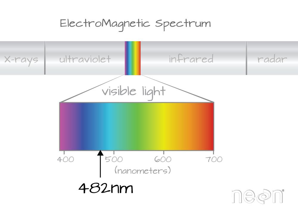
482 nanometers falls within the blue portion of the electromagnetic spectrum. Source: National Ecological Observatory Network
Band 21 has a associated wavelength center of 481.7982 nanometers (nm) which is in the blue portion (~380-500 nm) of the visible electromagnetic spectrum (~380-700 nm).
Bands and Wavelengths
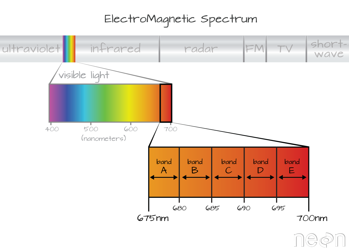
A band represents a group of wavelengths. For example, the wavelength values between 695 nm and 700 nm might be one band captured by an imaging spectrometer. The imaging spectrometer collects reflected light energy in a pixel for light in that band. Often when you work with a multi- or hyperspectral dataset, the band information is reported as the center wavelength value. This value represents the mean value of the wavelengths represented in that band. Thus in a band spanning 695-700 nm, the center would be 697.5 nm). The full width half max (FWHM) will also be reported. This value can be thought of as the spread of the band around that center point. So, a band that covers 800-805 nm might have a FWHM of 5 nm and a wavelength value of 802.5 nm.
Bands represent a range of values (types of light) within the electromagnetic spectrum. Values for each band are often represented as the center point value of each band. Source: National Ecological Observatory Network (NEON)
The HDF5 dataset that we are working with in this activity may contain more information than we need to work with. For example, we don't necessarily need to process all 426 bands available in a full NEON hyperspectral reflectance file - if we are interested in creating a product like NDVI which only uses bands in the Near InfraRed (NIR) and Red portions of the spectrum. Or we might only be interested in a spatial subset of the data - perhaps an area where we have collected corresponding ground data in the field.
The HDF5 format allows us to slice (or subset) the data - quickly extracting the subset that we need to process. Let's extract one of the green bands - band 34.
By the way - what is the center wavelength value associated with band 34?
Hint: wavelengths[34].
How do we know this band is a green band in the visible portion of the spectrum?
In order to effectively subset our data, let's first read the reflectance metadata stored as attributes in the "Reflectance_Data" dataset.
# First, we need to extract the reflectance metadata:

reflInfo <- h5readAttributes(h5_file, "/SJER/Reflectance/Reflectance_Data")

reflInfo

## $Cloud_conditions
## [1] "For cloud conditions information see Weather Quality Index dataset."
##
## $Cloud_type
## [1] "Cloud type may have been selected from multiple flight trajectories."
##
## $Data_Ignore_Value
## [1] -9999
##
## $Description
## [1] "Atmospherically corrected reflectance."
##
## $Dimension_Labels
## [1] "Line, Sample, Wavelength"
##
## $Dimensions
## [1] 1000 1000  426
##
## $Interleave
## [1] "BSQ"
##
## $Scale_Factor
## [1] 10000
##
## $Spatial_Extent_meters
## [1]  257000  258000 4112000 4113000
##
## $Spatial_Resolution_X_Y
## [1] 1 1
##
## $Units
## [1] "Unitless."
##
## $Units_Valid_range
## [1]     0 10000

# Next, we read the different dimensions


nRows <- reflInfo$Dimensions[1]

nCols <- reflInfo$Dimensions[2]

nBands <- reflInfo$Dimensions[3]


nRows

## [1] 1000

nCols

## [1] 1000

nBands

## [1] 426
The HDF5 read function reads data in the order: Bands, Cols, Rows. This is different from how R reads data. We'll adjust for this later.
# Extract or "slice" data for band 34 from the HDF5 file

b34 <- h5read(h5_file,"/SJER/Reflectance/Reflectance_Data",index=list(34,1:nCols,1:nRows))


# what type of object is b34?

class(b34)

## [1] "array"
A Note About Data Slicing in HDF5
Data slicing allows us to extract and work with subsets of the data rather than reading in the entire dataset into memory. In this example, we will extract and plot the green band without reading in all 426 bands. The ability to slice large datasets makes HDF5 ideal for working with big data.
Next, let's convert our data from an array (more than 2 dimensions) to a matrix (just 2 dimensions). We need to have our data in a matrix format to plot it.
# convert from array to matrix by selecting only the first band

b34 <- b34[1,,]


# display the class of this re-defined variable

class(b34)

## [1] "matrix" "array"
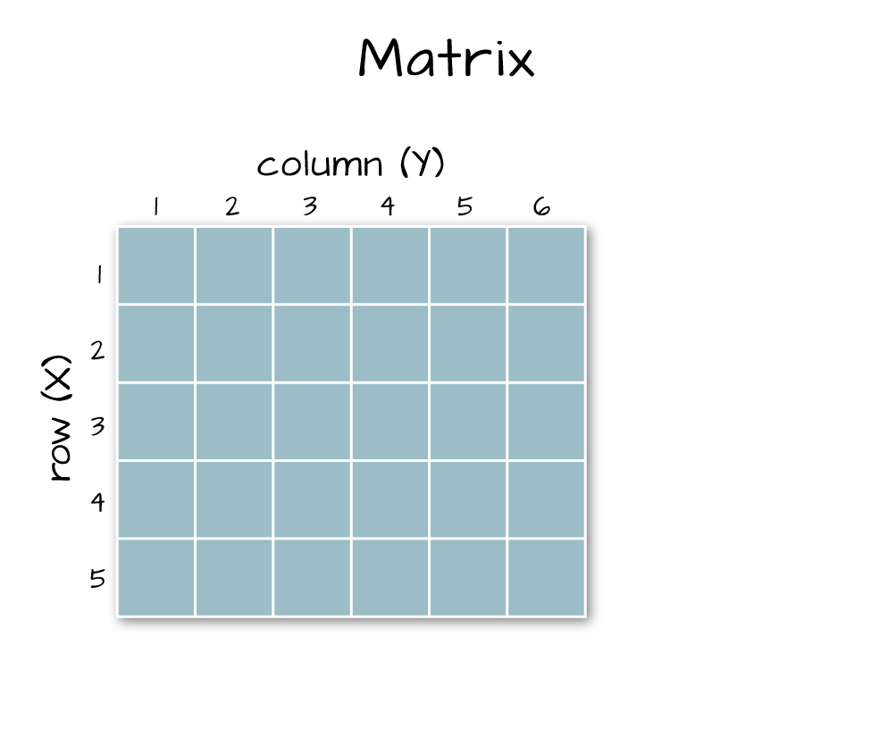
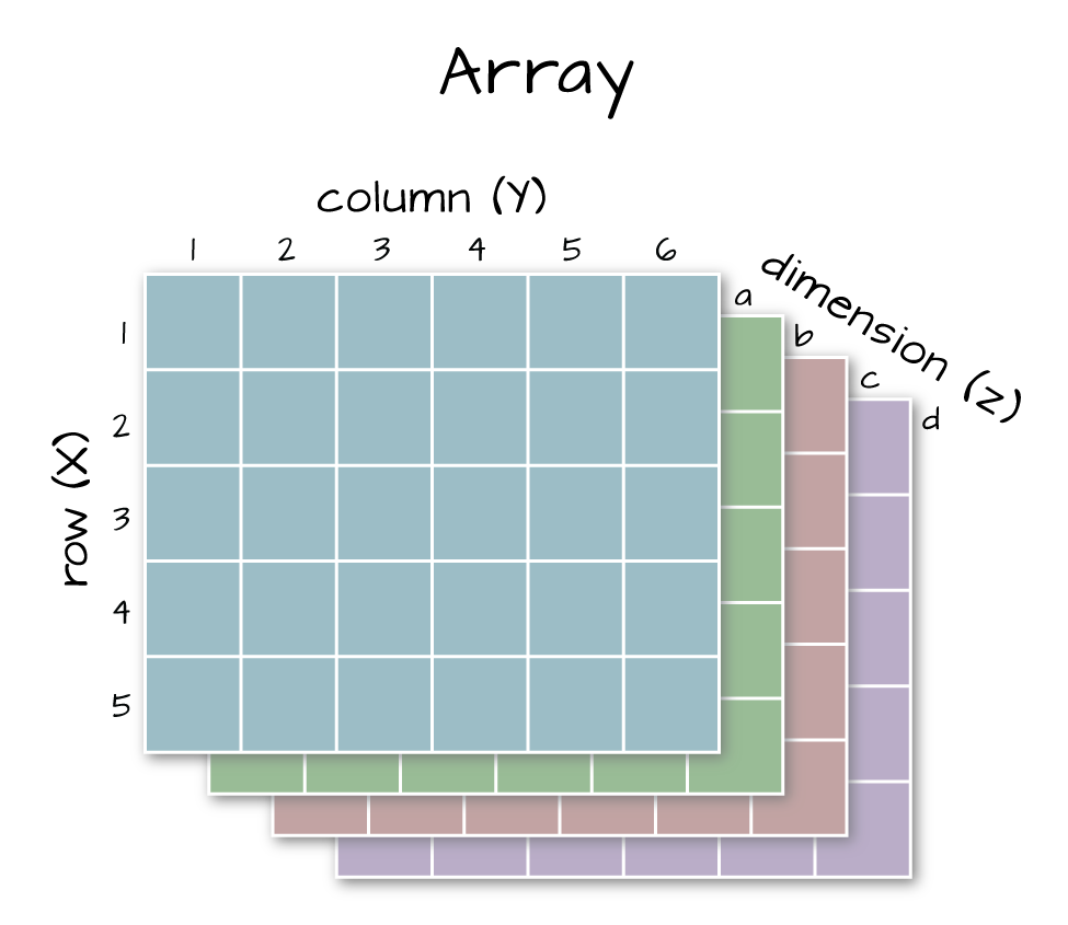
Arrays vs. Matrices
Arrays are matrices with more than 2 dimensions. When we say dimension, we are talking about the "z" associated with the data (imagine a series of tabs in a spreadsheet). Put the other way: matrices are arrays with only 2 dimensions. Arrays can have any number of dimensions one, two, ten or more.
Here is a matrix that is 4 x 3 in size (4 rows and 3 columns):
Metric
species 1
species 2
total number
23
45
average weight
14
5
average length
2.4
3.5
average height
32
12
Dimensions in Arrays
An array contains 1 or more dimensions in the "z" direction. For example, let's say that we collected the same set of species data for every day in a 30 day month. We might then have a matrix like the one above for each day for a total of 30 days making a 4 x 3 x 30 array (this dataset has more than 2 dimensions). More on R object types here (links to external site, DataCamp).
Left: a matrix has only 2 dimensions. Right: an array has more than 2 dimensions.
Next, let's look at the metadata for the reflectance data. When we do this, take note of 1) the scale factor and 2) the data ignore value. Then we can plot the band 34 data. Plotting spatial data as a visual "data check" is a good idea to make sure processing is being performed correctly and all is well with the image.
# look at the metadata for the reflectance dataset

h5readAttributes(h5_file,"/SJER/Reflectance/Reflectance_Data")

## $Cloud_conditions
## [1] "For cloud conditions information see Weather Quality Index dataset."
##
## $Cloud_type
## [1] "Cloud type may have been selected from multiple flight trajectories."
##
## $Data_Ignore_Value
## [1] -9999
##
## $Description
## [1] "Atmospherically corrected reflectance."
##
## $Dimension_Labels
## [1] "Line, Sample, Wavelength"
##
## $Dimensions
## [1] 1000 1000  426
##
## $Interleave
## [1] "BSQ"
##
## $Scale_Factor
## [1] 10000
##
## $Spatial_Extent_meters
## [1]  257000  258000 4112000 4113000
##
## $Spatial_Resolution_X_Y
## [1] 1 1
##
## $Units
## [1] "Unitless."
##
## $Units_Valid_range
## [1]     0 10000

# plot the image

image(b34)
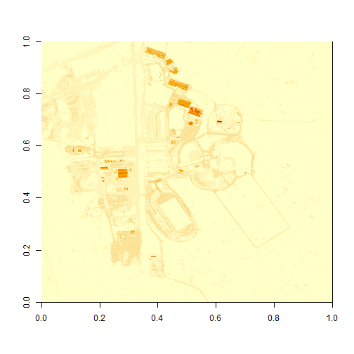
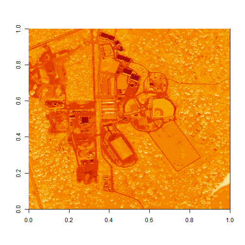
What do you notice about the first image? It's washed out and lacking any detail. What could be causing this? It got better when plotting the log of the values, but still not great.
# this is a little hard to visually interpret - what happens if we plot a log of the data?

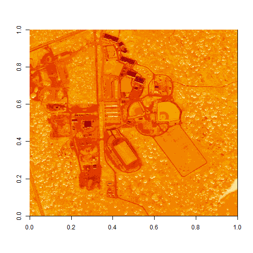
image(log(b34))
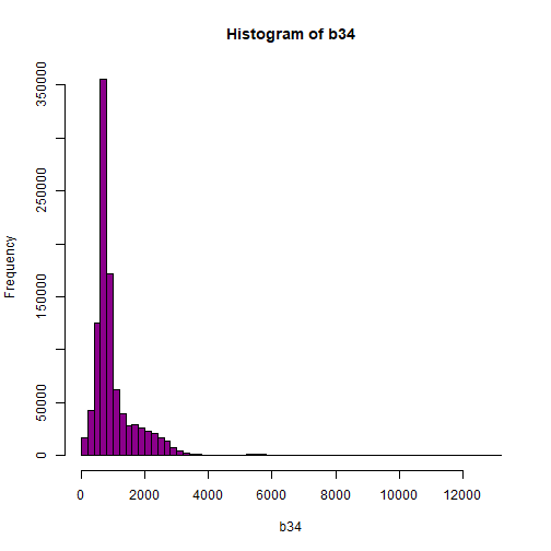
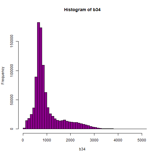
Let's look at the distribution of reflectance values in our data to figure out what is going on.
# Plot range of reflectance values as a histogram to view range

# and distribution of values.

hist(b34,breaks=50,col="darkmagenta")
# View values between 0 and 5000

hist(b34,breaks=100,col="darkmagenta",xlim = c(0, 5000))
As you're examining the histograms above, keep in mind that reflectance values range between 0-1. The data scale factor in the metadata tells us to divide all reflectance values by 10,000. Thus, a value of 5,000 equates to a reflectance value of 0.50. Storing data as integers (without decimal places) compared to floating points (with decimal places) creates a smaller file. This type of scaling is commin in remote sensing datasets.
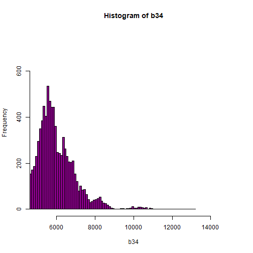
Notice in the data that there are some larger reflectance values (>5,000) that represent a smaller number of pixels. These pixels are skewing how the image renders.
Data Ignore Value
Image data in raster format will often contain a data ignore value and a scale factor. The data ignore value represents pixels where there are no data. Among other causes, no data values may be attributed to the sensor not collecting data in that area of the image or to processing results which yield null values.
Remember that the metadata for the Reflectance dataset designated -9999 as data ignore value. Thus, let's set all pixels with a value == -9999 to NA (no value). If we do this, R won't render these pixels.
# there is a no data value in our raster - let's define it

noDataValue <- as.numeric(reflInfo$Data_Ignore_Value)

noDataValue

## [1] -9999

# set all values equal to the no data value (-9999) to NA

b34[b34 == noDataValue] <- NA


# plot the image now

image(b34)
Reflectance Values and Image Stretch
Our image still looks dark because R is trying to render all reflectance values between 0 and 14999 as if they were distributed equally in the histogram. However we know they are not distributed equally. There are many more values between 0-5000 than there are values >5000.
Images contain a distribution of reflectance values. A typical image viewing program will render the values by distributing the entire range of reflectance values across a range of "shades" that the monitor can render - between 0 and 255.
However, often the distribution of reflectance values is not linear. For example, in the case of our data, most of the reflectance values fall between 0 and 0.5. Yet there are a few values >0.8 that are heavily impacting the way the image is
drawn on our monitor. Imaging processing programs like ENVI, QGIS and ArcGIS (and even Adobe Photoshop) allow you to adjust the stretch of the image. This is similar to adjusting the contrast and brightness in Photoshop.
The proper way to adjust our data would be to apply what's called an image stretch. We will learn how to stretch our image data later. For now, let's plot the values as the log function on the pixel reflectance values to factor out those larger values.
image(log(b34))
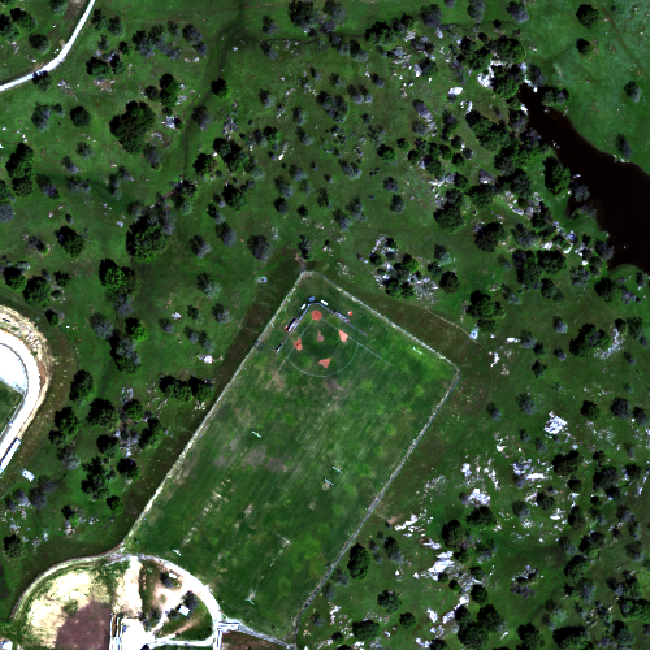
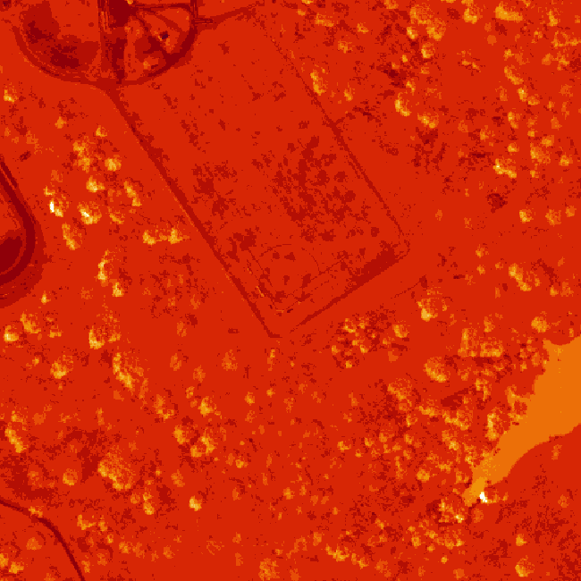
The log applied to our image increases the contrast making it look more like an image. However, look at the images below. The top one is an RGB image as the image should look. The bottom one is our log-adjusted image. Notice a difference?
Top: The image as it should look. Bottom: the image that we outputted from the code above. Notice a difference?
Transpose Image
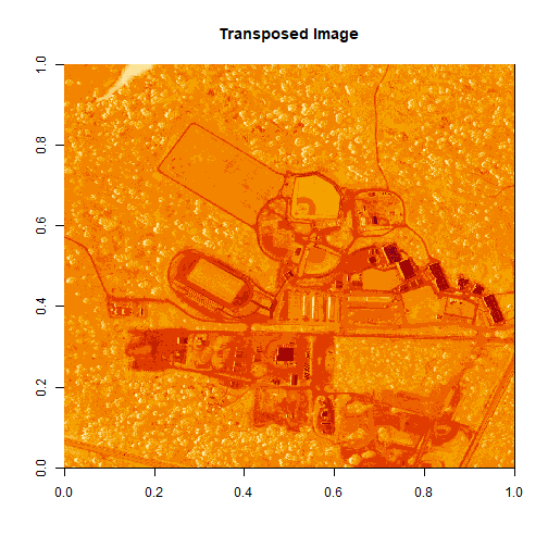
Notice that there are three data dimensions for this file: Bands x Rows x Columns. However, when R reads in the dataset, it reads them as: Columns x Bands x Rows. The data are flipped. We can quickly transpose the data to correct for this using the t or transpose command in R.
The orientation is rotated in our log adjusted image. This is because R reads in matrices starting from the upper left hand corner. While most rasters read pixels starting from the lower left hand corner. In the next section, we will deal with this issue by creating a proper georeferenced (spatially located) raster in R. The raster format will read in pixels following the same methods as other GIS and imaging processing software like QGIS and ENVI do.
# We need to transpose x and y values in order for our

# final image to plot properly

b34 <- t(b34)

image(log(b34), main="Transposed Image")
Create a Georeferenced Raster
Next, we will create a proper raster using the b34 matrix. The raster format will allow us to define and manage:
Image stretch
Coordinate reference system & spatial reference
Resolution
and other raster attributes...
It will also account for the orientation issue discussed above.
To create a raster in R, we need a few pieces of information, including:
The coordinate reference system (CRS)
The spatial extent of the image
Define Raster CRS
First, we need to define the Coordinate reference system (CRS) of the raster. To do that, we can first grab the EPSG code from the HDF5 attributes, and covert the EPSG to a CRS string. Then we can assign that CRS to the raster object.
# Extract the EPSG from the h5 dataset

h5EPSG <- h5read(h5_file, "/SJER/Reflectance/Metadata/Coordinate_System/EPSG Code")


# convert the EPSG code to a CRS string

h5CRS <- crs(paste0("+init=epsg:",h5EPSG))


# define final raster with projection info

# note that capitalization will throw errors on a MAC.

# if UTM is all caps it might cause an error!

b34r <- rast(b34,
        crs=h5CRS)


# view the raster attributes

b34r

## class       : SpatRaster
## size        : 1000, 1000, 1  (nrow, ncol, nlyr)
## resolution  : 1, 1  (x, y)
## extent      : 0, 1000, 0, 1000  (xmin, xmax, ymin, ymax)
## coord. ref. : WGS 84 / UTM zone 11N
## source(s)   : memory
## name        : lyr.1
## min value   :    32
## max value   : 13129

# let's have a look at our properly oriented raster. Take note of the

# coordinates on the x and y axis.


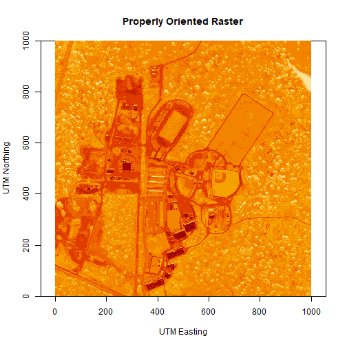
image(log(b34r),
      xlab = "UTM Easting",
      ylab = "UTM Northing",
      main = "Properly Oriented Raster")
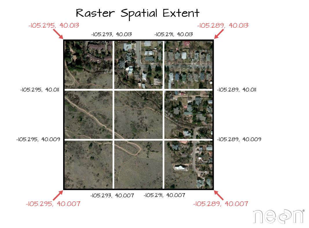
Next we define the extents of our raster. The extents will be used to calculate the raster's resolution. Fortunately, the spatial extent is provided in the HDF5 file "Reflectance_Data" group attributes that we saved before as reflInfo.
# Grab the UTM coordinates of the spatial extent

xMin <- reflInfo$Spatial_Extent_meters[1]

xMax <- reflInfo$Spatial_Extent_meters[2]

yMin <- reflInfo$Spatial_Extent_meters[3]

yMax <- reflInfo$Spatial_Extent_meters[4]


# define the extent (left, right, top, bottom)

rasExt <- ext(xMin,xMax,yMin,yMax)

rasExt

## SpatExtent : 257000, 258000, 4112000, 4113000 (xmin, xmax, ymin, ymax)

# assign the spatial extent to the raster

ext(b34r) <- rasExt


# look at raster attributes

b34r

## class       : SpatRaster
## size        : 1000, 1000, 1  (nrow, ncol, nlyr)
## resolution  : 1, 1  (x, y)
## extent      : 257000, 258000, 4112000, 4113000  (xmin, xmax, ymin, ymax)
## coord. ref. : WGS 84 / UTM zone 11N
## source(s)   : memory
## name        : lyr.1
## min value   :    32
## max value   : 13129
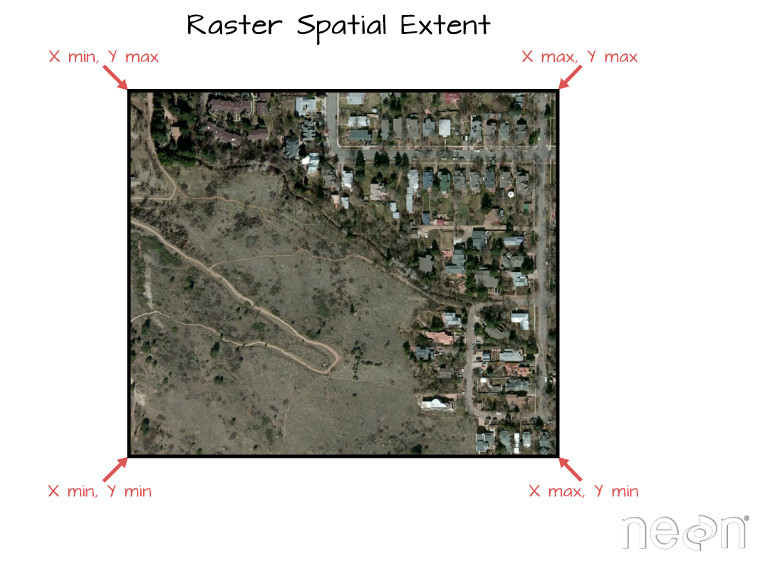
The extent of a raster represents the spatial location of each corner. The coordinate units will be determined by the spatial projection coordinate reference system that the data are in. Source: National Ecological Observatory Network (NEON)
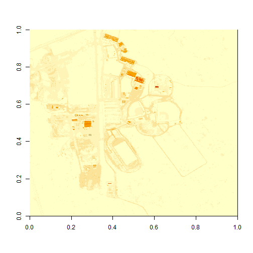
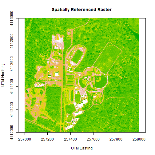
We can adjust the colors of our raster as well, if desired.
# let's change the colors of our raster and adjust the zlim

col <- terrain.colors(25)


image(b34r,
      xlab = "UTM Easting",
      ylab = "UTM Northing",
      main= "Spatially Referenced Raster",
      col=col,
      zlim=c(0,3000))
We've now created a raster from band 34 reflectance data. We can export the data as a raster, using the writeRaster command. Note that it's good practice to close the H5 connection before moving on!
# write out the raster as a geotiff

writeRaster(b34r,

            file=paste0(data_dir,"band34.tif"),

            overwrite=TRUE)


# close the H5 file

H5close()
Challenge: Work with Rasters
Try these three extensions on your own:
Create rasters using other bands in the dataset.
Vary the distribution of values in the image to mimic an image stretch.
e.g. b34[b34 > 6000 ] <- 6000
Use what you know to extract ALL of the reflectance values for ONE pixel rather than for an entire band. HINT: this will require you to pick
an x and y value and then all values in the z dimension: aPixel<- h5read(h5_file,"Reflectance",index=list(NULL,100,35)). Plot the spectra output.
In this tutorial, we will learn how to create multi (3) band images from hyperspectral data. We will also learn how to perform some basic raster calculations (known as raster math in the GIS world).
Learning Objectives
After completing this activity, you will be able to:
Extract a "slice" of data from a hyperspectral data cube.
Create a raster "stack" in R which can be used to create RGB images from band combinations in a hyperspectral data cube.
Plot data spatially on a map.
Create basic vegetation indices like NDVI using raster-based calculations in R.
Things You’ll Need To Complete This Tutorial
To complete this tutorial you will need the most current version of R and,
preferably, RStudio loaded on your computer. You will also need to create a NEON API token.
These hyperspectral remote sensing data provide information on the National Ecological Observatory Network'sSan Joaquin Experimental Range (SJER) field site in March of 2021. The data used in this lesson is the 1km by 1km mosaic tile named NEON_D17_SJER_DP3_257000_4112000_reflectance.h5. If you already completed the previous lesson in this tutorial series, you do not need to download this data again. The entire SJER reflectance dataset can be accessed from the NEON Data Portal.
R Script & Challenge Code: NEON data lessons often contain challenges to reinforce skills. If available, the code for challenge solutions is found in the downloadable R script of the entire lesson, available in the footer of each lesson page.
Recommended Skills
For this tutorial you should be comfortable working with HDF5 files that contain hyperspectral data, including reading in reflectance values and associated metadata and attributes.
We often want to generate a 3 band image from multi or hyperspectral data. The most commonly recognized band combination is RGB which stands for Red, Green and Blue. RGB images are just like an image that your camera takes. But other band combinations can be useful too. For example, near infrared images highlight healthy vegetation, which makes it easy to classify or identify where vegetation is located on the ground.
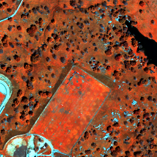
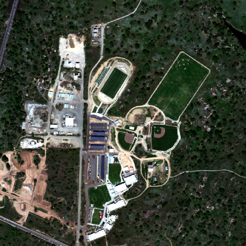
A portion of the SJER field site using red, green and blue (bands 58, 34, and 19).Here is the same section of SJER but with other bands highlighted to create a colored infrared image – near infrared, green and blue (bands 90, 34, and 19).
Data Tip - Band Combinations: The Biodiversity Informatics group created a great interactive tool that lets you explore band combinations. Check it out. Learn more about band combinations using a great online tool from the American Museum of Natural History! (The tool requires Flash player.)
Create a Raster Stack in R
In the previous lesson, we exported a single band of the NEON Reflectance data from a HDF5 file. In this activity, we will create a full color image using 3 (red, green and blue - RGB) bands. We will follow many of the steps we followed in the Intro to Working with Hyperspectral Remote Sensing Data in HDF5 Format in R tutorial.
These steps included loading required packages, downloading the data (optionally, you don't need to do this if you downloaded the data from the previous lesson), and reading in our file and viewing the hdf5 file structure.
First, let's load the required R packages, terra and rhdf5, and read in our token.
As of June 2026, NEON requires an API token for data downloads, to reduce bot scraping and improve user support. Tokens can be generated in NEON data portal user accounts - log in to your account or create one, and go to the API Tokens section. For best practices in storing and using tokens, follow the instructions here.
Next set the working directory to ensure R can find the file we wish to import.
Be sure to move the download into your working directory!
# set data directory (this will depend on your local environment)
data_dir <- "~/data/"
We can use the neonUtilities function byTileAOP to download a single reflectance tile. You can run help(byTileAOP) to see more details on what the various inputs are. For this exercise, we'll specify the UTM Easting and Northing to be (257500, 4112500), which will download the tile with the lower left corner (257000, 4112000).
## Successfully downloaded 1 files to ~/data//DP3.30006.001
This file will be downloaded into a nested subdirectory under the ~/data folder, inside a folder named DP3.30006.001 (the Data Product ID). The file should show up in this location: ~/data/DP3.30006.001/neon-aop-products/2021/FullSite/D17/2021_SJER_5/L3/Spectrometer/Reflectance/NEON_D17_SJER_DP3_257000_4112000_reflectance.h5.
Now we can read in the file. You can move this file to a different location, but make sure to change the path accordingly.
# Define the h5 file name to be opened

h5_file <- paste0(data_dir,"DP3.30006.001/neon-aop-products/2021/FullSite/D17/2021_SJER_5/L3/Spectrometer/Reflectance/NEON_D17_SJER_DP3_257000_4112000_reflectance.h5")
As in the last lesson, let's use View(h5ls) to take a look inside this hdf5 dataset:
View(h5ls(h5_file,all=T))
To spatially locate our raster data, we need a few key attributes:
The coordinate reference system
The spatial extent of the raster
We'll begin by grabbing these key attributes from the H5 file.
# define coordinate reference system from the EPSG code provided in the HDF5 file
h5EPSG <- h5read(h5_file,"/SJER/Reflectance/Metadata/Coordinate_System/EPSG Code" )
h5CRS <- crs(paste0("+init=epsg:",h5EPSG))

# get the Reflectance_Data attributes
reflInfo <- h5readAttributes(h5_file,"/SJER/Reflectance/Reflectance_Data" )

# Grab the UTM coordinates of the spatial extent
xMin <- reflInfo$Spatial_Extent_meters[1]
xMax <- reflInfo$Spatial_Extent_meters[2]
yMin <- reflInfo$Spatial_Extent_meters[3]
yMax <- reflInfo$Spatial_Extent_meters[4]

# define the extent (left, right, top, bottom)
rastExt <- ext(xMin,xMax,yMin,yMax)

# view the extent to make sure that it looks right
rastExt

## SpatExtent : 257000, 258000, 4112000, 4113000 (xmin, xmax, ymin, ymax)

# Finally, define the no data value for later
h5NoDataValue <- as.integer(reflInfo$Data_Ignore_Value)
cat('No Data Value:',h5NoDataValue)

## No Data Value: -9999
The function band2Rast slices a band of data from the HDF5 file, and extracts the reflectance array for that band. It then converts the data into a matrix, converts it to a raster, and finally returns a spatially corrected raster for the specified band.
The function requires the following variables:
file: the hdf5 reflectance file
band: the band number we wish to extract
noDataValue: the noDataValue for the raster
extent: a terra spatial extent (SpatExtent) object .
crs: the Coordinate Reference System for the raster
The function output is a spatially referenced, R terra object.
# file: the hdf5 file
# band: the band you want to process
# returns: a matrix containing the reflectance data for the specific band

band2Raster <- function(file, band, noDataValue, extent, CRS){
    # first, read in the raster
    out <- h5read(file,"/SJER/Reflectance/Reflectance_Data",index=list(band,NULL,NULL))
	  # Convert from array to matrix
	  out <- (out[1,,])
	  # transpose data to fix flipped row and column order
    # depending upon how your data are formatted you might not have to perform this
    # step.
	  out <- t(out)
    # assign data ignore values to NA
    # note, you might chose to assign values of 15000 to NA
    out[out == noDataValue] <- NA

    # turn the out object into a raster
    outr <- rast(out,crs=CRS)

    # assign the extents to the raster
    ext(outr) <- extent

    # return the terra raster object
    return(outr)
}
Now that the function is created, we can create our list of rasters. The list
specifies which bands (or dimensions in our hyperspectral dataset) we want to
include in our raster stack. Let's start with a typical RGB (red, green, blue)
combination. We will use bands 14, 9, and 4 (bands 58, 34, and 19 in a full
NEON hyperspectral dataset).
Data Tip - wavelengths and bands: Remember that
you can look at the wavelengths dataset in the HDF5 file to determine the center
wavelength value for each band. Keep in mind that this data subset only includes
every fourth band that is available in a full NEON hyperspectral dataset!
# create a list of the bands (R,G,B) we want to include in our stack
rgb <- list(58,34,19)

# lapply tells R to apply the function to each element in the list

rgb_rast <- lapply(rgb,FUN=band2Raster, file = h5_file,
                   noDataValue=h5NoDataValue,
                   ext=rastExt,
                   CRS=h5CRS)
Check out the properties or rgb_rast:
rgb_rast

## [[1]]
## class       : SpatRaster
## size        : 1000, 1000, 1  (nrow, ncol, nlyr)
## resolution  : 1, 1  (x, y)
## extent      : 257000, 258000, 4112000, 4113000  (xmin, xmax, ymin, ymax)
## coord. ref. : WGS 84 / UTM zone 11N
## source(s)   : memory
## name        : lyr.1
## min value   :     0
## max value   : 14950
##
## [[2]]
## class       : SpatRaster
## size        : 1000, 1000, 1  (nrow, ncol, nlyr)
## resolution  : 1, 1  (x, y)
## extent      : 257000, 258000, 4112000, 4113000  (xmin, xmax, ymin, ymax)
## coord. ref. : WGS 84 / UTM zone 11N
## source(s)   : memory
## name        : lyr.1
## min value   :    32
## max value   : 13129
##
## [[3]]
## class       : SpatRaster
## size        : 1000, 1000, 1  (nrow, ncol, nlyr)
## resolution  : 1, 1  (x, y)
## extent      : 257000, 258000, 4112000, 4113000  (xmin, xmax, ymin, ymax)
## coord. ref. : WGS 84 / UTM zone 11N
## source(s)   : memory
## name        : lyr.1
## min value   :     9
## max value   : 11802
Note that it displays properties of 3 rasters. Finally, we can create a raster stack from our list of rasters as follows:
rgbStack <- rast(rgb_rast)
In the code chunk above, we used the lapply() function, which is a powerful, flexible way to apply a function (in this case, our band2Raster() function) multiple times. You can learn more about lapply() here.
NOTE: We are using the raster stack object in R to store several rasters that are of the same CRS and extent. This is a popular and convenient way to organize co-incident rasters.
Next, add the names of the bands to the raster so we can easily keep track of the bands in the list.
# Create a list of band names
bandNames <- paste("Band_",unlist(rgb),sep="")

# set the rasterStack's names equal to the list of bandNames created above
names(rgbStack) <- bandNames

# check properties of the raster list - note the band names
rgbStack

## class       : SpatRaster
## size        : 1000, 1000, 3  (nrow, ncol, nlyr)
## resolution  : 1, 1  (x, y)
## extent      : 257000, 258000, 4112000, 4113000  (xmin, xmax, ymin, ymax)
## coord. ref. : WGS 84 / UTM zone 11N
## source(s)   : memory
## names       : Band_58, Band_34, Band_19
## min values  :       0,      32,       9
## max values  :   14950,   13129,   11802


# scale the data as specified in the reflInfo$Scale Factor
rgbStack <- rgbStack/as.integer(reflInfo$Scale_Factor)

# plot one raster in the stack to make sure things look OK.
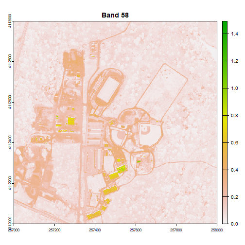
plot(rgbStack$Band_58, main="Band 58")
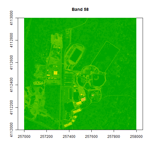
We can play with the color ramps too if we want:
# change the colors of our raster
colors1 <- terrain.colors(25)
image(rgbStack$Band_58, main="Band 58", col=colors1)
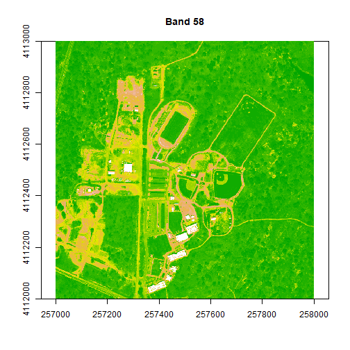
# adjust the zlims or the stretch of the image
image(rgbStack$Band_58, main="Band 58", col=colors1, zlim = c(0,.5))
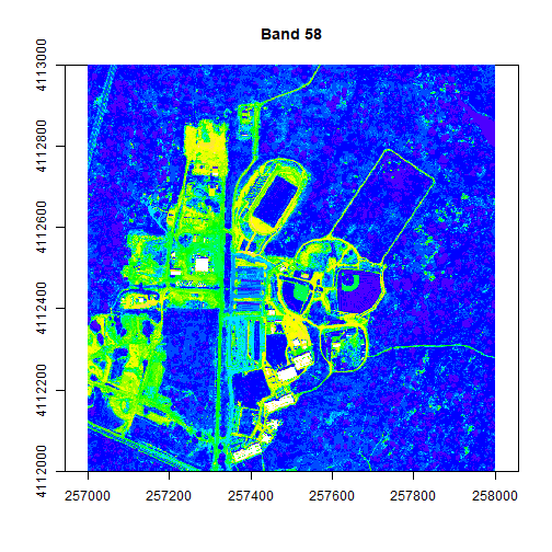
# try a different color palette
colors2 <- topo.colors(15, alpha = 1)
image(rgbStack$Band_58, main="Band 58", col=colors2, zlim=c(0,.5))
The plotRGB function allows you to combine three bands to create an true-color image.
# create a 3 band RGB image
plotRGB(rgbStack,
        r=1,g=2,b=3,
        stretch = "lin")
A note about image stretching: Notice that we use the argument stretch="lin" in this plotting function, which automatically stretches the brightness values for us to produce a natural-looking image.
Once you've created your raster, you can export it as a GeoTIFF using writeRaster. You can bring this GeoTIFF into any GIS software, such as QGIS or ArcGIS.
# Write out final raster
# Note: if you set overwrite to TRUE, then you will overwrite (and lose) any older version of the tif file!
writeRaster(rgbStack, file=paste0(data_dir,"NEON_D17_SJER_DP3_257000_4112000_reflectance_2021_RGB.tif"), overwrite=TRUE)
Data Tip - False color and near infrared images:
Use the band combinations listed at the top of this page to modify the raster list.
What type of image do you get when you change the band values?
Challenge: Other band combinations
Use different band combinations to create other "RGB" images. Suggested band combinations are below for use with the full NEON hyperspectral reflectance datasets (for this example dataset, divide the band number by 4 and round to the nearest whole number):
Color Infrared/False Color: rgb (90,34,19)
SWIR, NIR, Red Band: rgb (152,90,58)
False Color: rgb (363,246,55)
Raster Math - Creating NDVI and other Vegetation Indices in R
In this last part, we will calculate some vegetation indices using raster math in R! We will start by creating NDVI or Normalized Difference Vegetation Index.
About NDVI
NDVI is a ratio between the near infrared (NIR) portion of the electromagnetic spectrum and the red portion of the spectrum.
$$
NDVI = \frac{NIR-RED}{NIR+RED}
$$
Please keep in mind that there are different ways to aggregate bands when using hyperspectral data. This example is using individual bands to perform the NDVI calculation. Using individual bands is not necessarily the best way to calculate NDVI from hyperspectral data.
# Calculate NDVI
# select bands to use in calculation (red, NIR)
ndviBands <- c(58,90)

# create raster list and then a stack using those two bands
ndviRast <- lapply(ndviBands,FUN=band2Raster, file = h5_file,
                   noDataValue=h5NoDataValue,
                   ext=rastExt, CRS=h5CRS)

ndviStack <- rast(ndviRast)

# make the names pretty
bandNDVINames <- paste("Band_",unlist(ndviBands),sep="")
names(ndviStack) <- bandNDVINames

# view the properties of the new raster stack

ndviStack

## class       : SpatRaster
## size        : 1000, 1000, 2  (nrow, ncol, nlyr)
## resolution  : 1, 1  (x, y)
## extent      : 257000, 258000, 4112000, 4113000  (xmin, xmax, ymin, ymax)
## coord. ref. : WGS 84 / UTM zone 11N
## source(s)   : memory
## names       : Band_58, Band_90
## min values  :       0,      11
## max values  :   14950,   14887

#calculate NDVI

NDVI <- function(x) {
	  (x[,2]-x[,1])/(x[,2]+x[,1])
}

ndviCalc <- app(ndviStack,NDVI)

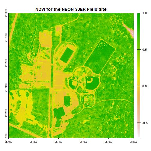
plot(ndviCalc, main="NDVI for the NEON SJER Field Site")
# Now, play with breaks and colors to create a meaningful map
# add a color map with 4 colors

myCol <- rev(terrain.colors(4)) # use the 'rev()' function to put green as the highest NDVI value
# add breaks to the colormap, including lowest and highest values (4 breaks = 3 segments)

brk <- c(0, .25, .5, .75, 1)

# plot the image using breaks
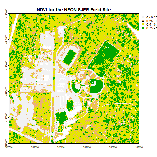
plot(ndviCalc, main="NDVI for the NEON SJER Field Site", col=myCol, breaks=brk)
Challenge: Work with Indices
Try the following on your own:
Calculate the Normalized Difference Nitrogen Index (NDNI) using the following equation:
$$
NDNI = \frac{log(\frac{1}{p_{1510}}) - log(\frac{1}{p_{1680}})}{log(\frac{1}{p_{1510}}) + log(\frac{1}{p_{1680}})}
$$
2. Calculate the Enhanced Vegetation Index (EVI). Hint: Look up the formula, and apply the appropriate NEON bands. Hint: You can look at satellite datasets, such as USGS Landsat EVI.
Explore the bands in the hyperspectral data. What happens if you average reflectance values across multiple Red and NIR bands and then calculate NDVI?
The LiDAR and imagery data used to create the rasters in this dataset were
collected over the San Joaquin field site located in California (NEON Domain 17)
and processed at NEON
headquarters. The entire dataset can be accessed by request from the NEON website.
This data download contains several files used in related tutorials. The path to
the files we will be using in this tutorial is:
NEON-DS-Field-Site-Spatial-Data/SJER/.
You should set your working directory to the parent directory of the downloaded
data to follow the code exactly.
Raster or "gridded" data are data that are saved in pixels. In the spatial world,
each pixel represents an area on the Earth's surface. For example in the raster
below, each pixel represents a particular land cover class that would be found in
that location in the real world.
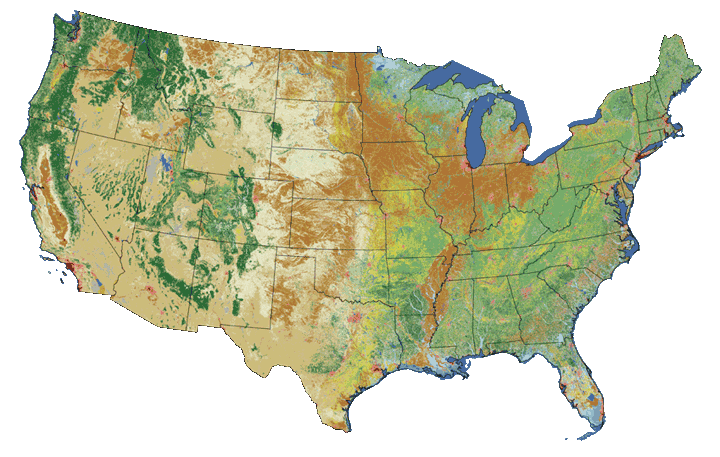
The National Land Cover dataset (NLCD) is an example of a commonly used
raster dataset. Each pixel in the Landsat derived raster represents a land cover
class. Source: Multi-Resolution Land Characteristics Consortium.
To work with rasters in R, we need two key packages, sp and raster.
To install the raster package you can use install.packages('raster').
When you install the raster package, sp should also install. Also install the
rgdal package install.packages('rgdal'). Among other things, rgdal will
allow us to export rasters to GeoTIFF format.
Once installed we can load the packages and start working with raster data.
# load the raster, sp, and rgdal packages
library(raster)
library(sp)
library(rgdal)

# set working directory to data folder
#setwd("pathToDirHere")
wd <- ("~/Git/data/")
setwd(wd)
Next, let's load a raster containing elevation data into our environment. And
look at the attributes.
# load raster in an R object called 'DEM'
DEM <- raster(paste0(wd, "NEON-DS-Field-Site-Spatial-Data/SJER/DigitalTerrainModel/SJER2013_DTM.tif"))

# look at the raster attributes.
DEM

## class      : RasterLayer
## dimensions : 5060, 4299, 21752940  (nrow, ncol, ncell)
## resolution : 1, 1  (x, y)
## extent     : 254570, 258869, 4107302, 4112362  (xmin, xmax, ymin, ymax)
## crs        : +proj=utm +zone=11 +datum=WGS84 +units=m +no_defs
## source     : /Users/olearyd/Git/data/NEON-DS-Field-Site-Spatial-Data/SJER/DigitalTerrainModel/SJER2013_DTM.tif
## names      : SJER2013_DTM
Notice a few things about this raster.
dimensions: the "size" of the file in pixels
nrow, ncol: the number of rows and columns in the data (imagine a spreadsheet or a matrix).
ncells: the total number of pixels or cells that make up the raster.
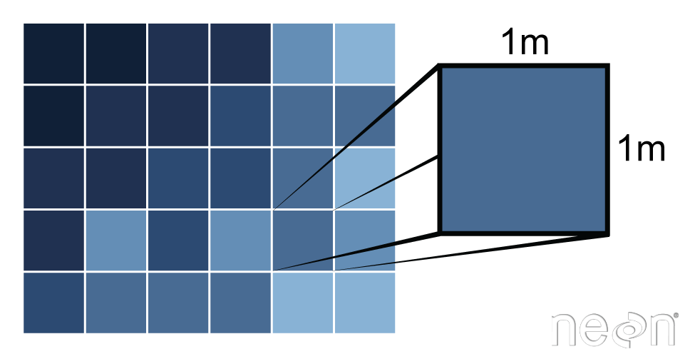
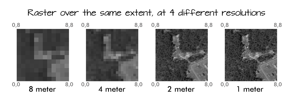
resolution: the size of each pixel (in meters in this case). 1 meter pixels
means that each pixel represents a 1m x 1m area on the earth's surface.
extent: the spatial extent of the raster. This value will be in the same
coordinate units as the coordinate reference system of the raster.
coord ref: the coordinate reference system string for the raster. This
raster is in UTM (Universal Trans Mercator) zone 11 with a datum of WGS 84.
More on UTM here.
Work with Rasters in R
Now that we have the raster loaded into R, let's grab some key raster attributes.
Define Min/Max Values
By default this raster doesn't have the min or max values associated with it's attributes
Let's change that by using the setMinMax() function.
# calculate and save the min and max values of the raster to the raster object
DEM <- setMinMax(DEM)

# view raster attributes
DEM

## class      : RasterLayer
## dimensions : 5060, 4299, 21752940  (nrow, ncol, ncell)
## resolution : 1, 1  (x, y)
## extent     : 254570, 258869, 4107302, 4112362  (xmin, xmax, ymin, ymax)
## crs        : +proj=utm +zone=11 +datum=WGS84 +units=m +no_defs
## source     : /Users/olearyd/Git/data/NEON-DS-Field-Site-Spatial-Data/SJER/DigitalTerrainModel/SJER2013_DTM.tif
## names      : SJER2013_DTM
## values     : 228.1, 518.66  (min, max)
Notice the values is now part of the attributes and shows the min and max values
for the pixels in the raster. What these min and max values represent depends on
what is represented by each pixel in the raster.
You can also view the rasters min and max values and the range of values contained
within the pixels.
#Get min and max cell values from raster
#NOTE: this code may fail if the raster is too large
cellStats(DEM, min)

## [1] 228.1

cellStats(DEM, max)

## [1] 518.66

cellStats(DEM, range)

## [1] 228.10 518.66
View CRS
First, let's consider the Coordinate Reference System (CRS).
We can also create a histogram to view the distribution of values in our raster.
Note that the max number of pixels that R will plot by default is 100,000. We
can tell it to plot more using the maxpixels attribute. Be careful with this,
if your raster is large this can take a long time or crash your program.
Since our raster is a digital elevation model, we know that each pixel contains
elevation data about our area of interest. In this case the units are meters.
This is an easy and quick data checking tool. Are there any totally weird values?
# the distribution of values in the raster
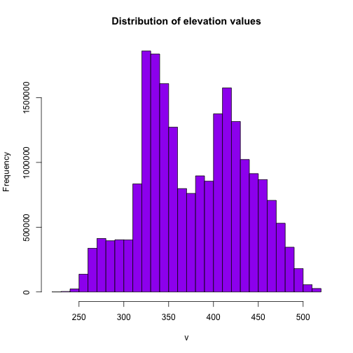
hist(DEM, main="Distribution of elevation values",
     col= "purple",
     maxpixels=22000000)
It looks like we have a lot of land around 325m and 425m.
Plot Raster Data
Let's take a look at our raster now that we know a bit more about it. We can do
a simple plot with the plot() function.
# plot the raster
# note that this raster represents a small region of the NEON SJER field site
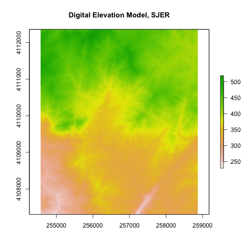
plot(DEM,
		 main="Digital Elevation Model, SJER") # add title with main
R has an image() function that allows you to control the way a raster is
rendered on the screen. The plot() function in R has a base setting for the number
of pixels that it will plot (100,000 pixels). The image command thus might be
better for rendering larger rasters.
# create a plot of our raster
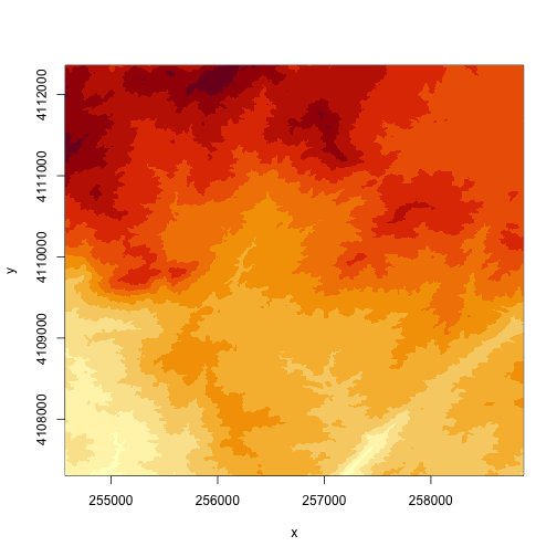
image(DEM)
# specify the range of values that you want to plot in the DEM
# just plot pixels between 250 and 300 m in elevation
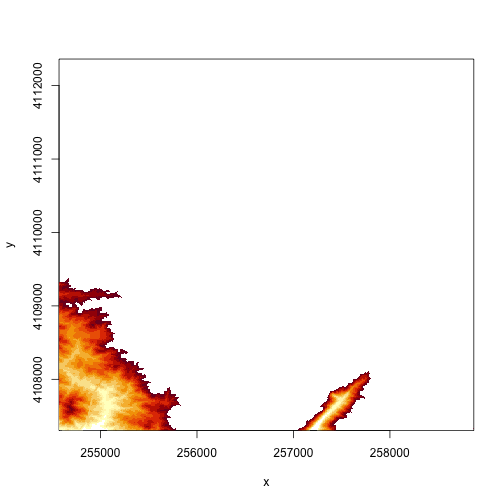
image(DEM, zlim=c(250,300))
# we can specify the colors too
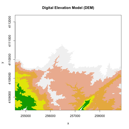
col <- terrain.colors(5)
image(DEM, zlim=c(250,375), main="Digital Elevation Model (DEM)", col=col)
Plotting with Colors
In the above example. terrain.colors() tells R to create a palette of colors
within the terrain.colors color ramp. There are other palettes that you can
use as well include rainbow and heat.colors.
What happens if you change the number of colors in the terrain.colors() function?
What happens if you change the zlim values in the image() function?
What are the other attributes that you can specify when using the image() function?
Breaks and Colorbars in R
A digital elevation model (DEM) is an example of a continuous raster. It
contains elevation values for a range. For example, elevations values in a
DEM might include any set of values between 200 m and 500 m. Given this range,
you can plot DEM pixels using a gradient of colors.
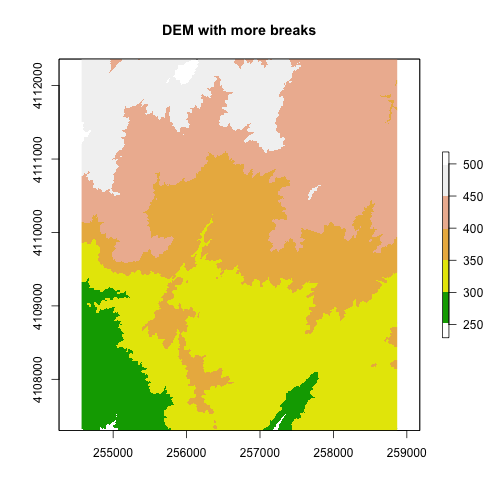
By default, R will assign the gradient of colors uniformly across the full
range of values in the data. In our case, our DEM has values between 250 and 500.
However, we can adjust the "breaks" which represent the numeric locations where
the colors change if we want too.
# add a color map with 5 colors
col=terrain.colors(5)

# add breaks to the colormap (6 breaks = 5 segments)
brk <- c(250, 300, 350, 400, 450, 500)

plot(DEM, col=col, breaks=brk, main="DEM with more breaks")
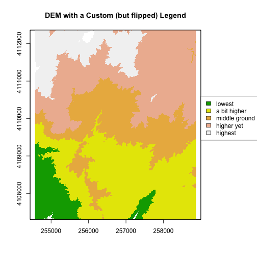
We can also customize the legend appearance.
# First, expand right side of clipping rectangle to make room for the legend
# turn xpd off
par(xpd = FALSE, mar=c(5.1, 4.1, 4.1, 4.5))

# Second, plot w/ no legend
plot(DEM, col=col, breaks=brk, main="DEM with a Custom (but flipped) Legend", legend = FALSE)

# Third, turn xpd back on to force the legend to fit next to the plot.
par(xpd = TRUE)

# Fourth, add a legend - & make it appear outside of the plot
legend(par()$usr[2], 4110600,
        legend = c("lowest", "a bit higher", "middle ground", "higher yet", "highest"),
        fill = col)
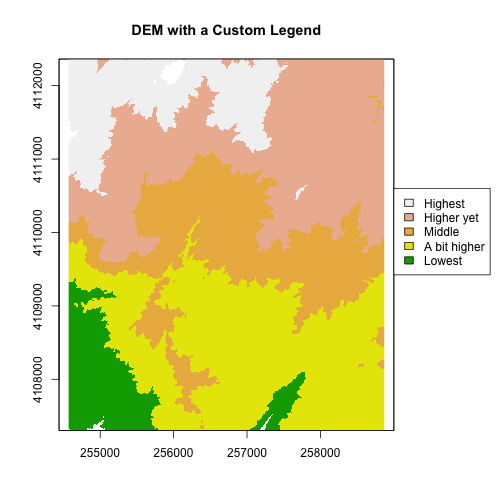
Notice that the legend is in reverse order in the previous plot. Let’s fix that.
We need to both reverse the order we have the legend laid out and reverse the
the color fill with the rev() colors.
# Expand right side of clipping rect to make room for the legend
par(xpd = FALSE,mar=c(5.1, 4.1, 4.1, 4.5))
#DEM with a custom legend
plot(DEM, col=col, breaks=brk, main="DEM with a Custom Legend",legend = FALSE)
#turn xpd back on to force the legend to fit next to the plot.
par(xpd = TRUE)

#add a legend - but make it appear outside of the plot
legend( par()$usr[2], 4110600,
        legend = c("Highest", "Higher yet", "Middle","A bit higher", "Lowest"),
        fill = rev(col))
Try the code again but only make one of the changes -- reverse order or reverse
colors-- what happens?
The raster plot now inverts the elevations! This is a good reason to understand
your data so that a simple visualization error doesn't have you reversing the
slope or some other error.
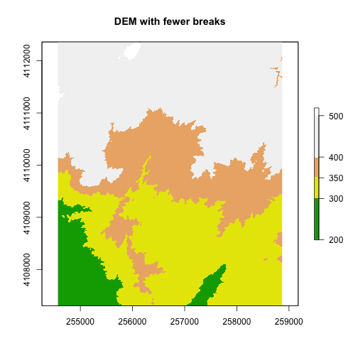
We can add a custom color map with fewer breaks as well.
#add a color map with 4 colors
col=terrain.colors(4)
#add breaks to the colormap (6 breaks = 5 segments)
brk <- c(200, 300, 350, 400,500)
plot(DEM, col=col, breaks=brk, main="DEM with fewer breaks")
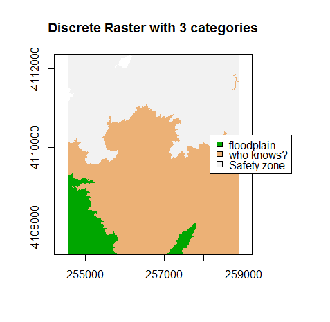
A discrete dataset has a set of unique categories or classes. One example could
be land use classes. The example below shows elevation zones generated using the
same DEM.
A DEM with discrete classes. In this case, the classes relate to regions of elevation values.
Basic Raster Math
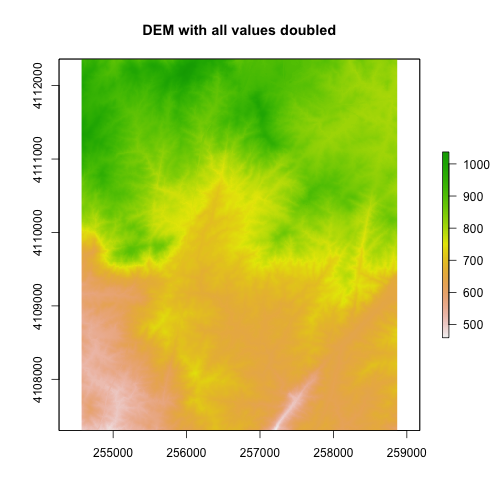
We can also perform calculations on our raster. For instance, we could multiply
all values within the raster by 2.
#multiple each pixel in the raster by 2
DEM2 <- DEM * 2

DEM2

## class      : RasterLayer
## dimensions : 5060, 4299, 21752940  (nrow, ncol, ncell)
## resolution : 1, 1  (x, y)
## extent     : 254570, 258869, 4107302, 4112362  (xmin, xmax, ymin, ymax)
## crs        : +proj=utm +zone=11 +datum=WGS84 +units=m +no_defs
## source     : memory
## names      : SJER2013_DTM
## values     : 456.2, 1037.32  (min, max)

#plot the new DEM
plot(DEM2, main="DEM with all values doubled")
Cropping Rasters in R
You can crop rasters in R using different methods. You can crop the raster directly
drawing a box in the plot area. To do this, first plot the raster. Then define
the crop extent by clicking twice:
Click in the UPPER LEFT hand corner where you want the crop
box to begin.
Click again in the LOWER RIGHT hand corner to define where the box ends.
You'll see a red box on the plot. NOTE that this is a manual process that can be
used to quickly define a crop extent.
#plot the DEM
plot(DEM)

#Define the extent of the crop by clicking on the plot
cropbox1 <- drawExtent()

#crop the raster, then plot the new cropped raster
DEMcrop1 <- crop(DEM, cropbox1)

#plot the cropped extent
plot(DEMcrop1)
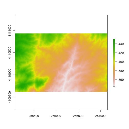
You can also manually assign the extent coordinates to be used to crop a raster.
We'll need the extent defined as (xmin, xmax, ymin , ymax) to do this.
This is how we'd crop using a GIS shapefile (with a rectangular shape)
#define the crop extent
cropbox2 <-c(255077.3,257158.6,4109614,4110934)
#crop the raster
DEMcrop2 <- crop(DEM, cropbox2)
#plot cropped DEM
plot(DEMcrop2)
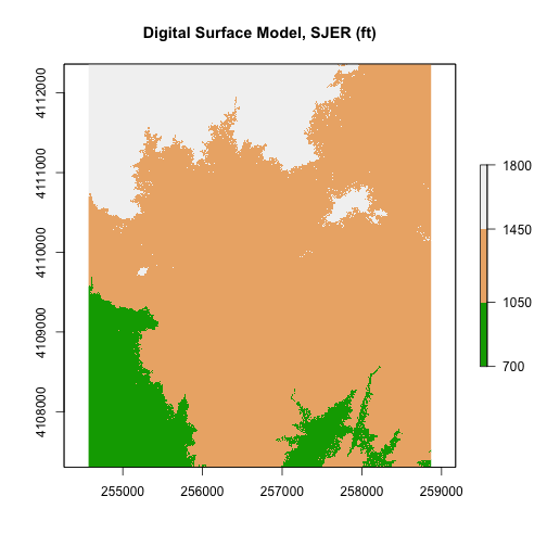
### Challenge: Plot a Digital Surface Model
Use what you've learned to open and plot a Digital Surface Model.
Create an R object called DSM from the raster: DigitalSurfaceModel/SJER2013_DSM.tif.
Convert the raster data from m to feet. What is that conversion again? Oh, right 1m = ~3.3ft.
Plot the DSM in feet using a custom color map.
Create numeric breaks that make sense given the distribution of the data.
Hint, your breaks might represent high elevation, medium elevation,
low elevation.
In this tutorial you will use the free HDFView tool to explore HDF5 files and
the groups and datasets contained within. You will also see how HDF5 files can
be structured and explore metadata using both spatial and temporal data stored
in HDF5!
Learning Objectives
After completing this activity, you will be able to:
Explain how data can be structured and stored in HDF5 format.
Navigate to metadata in an HDF5 file, making it "self describing".
Explore HDF5 files using the free HDFView application.
Tools You Will Need
Install the free HDFView application. This application allows you to explore the contents of an HDF5 file easily.
Click here to go to the download page.
Select the HDFView download option that matches the operating system
(Mac OS X, Windows, or Linux) and computer setup (32 bit vs 64 bit) that you have.
Hierarchical Data Format 5 - HDF5
Hierarchical Data Format version 5 (HDF5), is an open file format that supports
large, complex, heterogeneous data. Some key points about HDF5:
HDF5 uses a "file directory" like structure.
The HDF5 data models organizes information using Groups. Each group may contain one or more datasets.
HDF5 is a self describing file format. This means that the metadata for the
data contained within the HDF5 file, are built into the file itself.
One HDF5 file may contain several heterogeneous data types (e.g. images,
numeric data, data stored as strings).
In this tutorial, we will explore two different types of data saved in HDF5.
This will allow us to better understand how one file can store multiple different
types of data, in different ways.
Part 1: Exploring Hyperspectral Imagery stored in HDF5
NEON airborne observation platform.
First, we will explore a hyperspectral dataset, collected by the
NEON Airborne Observation Platform (AOP)
and saved in HDF5 format. In the hyperpsectral data cubes, each pixel in the dataset contains reflectance values for hundreds of bands (426) collected by the sensor.
A few notes about hyperspectral imagery:
An imaging spectrometer, which collects hyperspectral imagery, records light energy reflected off objects on the earth's surface.
The data are inherently spatial. Each pixel in the image is located spatially and represents an area of ground on the earth.
Similar to an RGB (Red, Green, Blue) camera, an imaging spectrometer records reflected light energy. Each pixel contain several hundred bands of reflectance data.
A hyperspectral instrument records reflected light energy across very narrow bands. The NEON Imaging Spectrometer collects 426 bands of information for each pixel on the ground.
Read more about hyperspectral remote sensing data:
Let's open some hyperspectral imagery stored in HDF5 format to see what the file
structure can like for a different type of data.
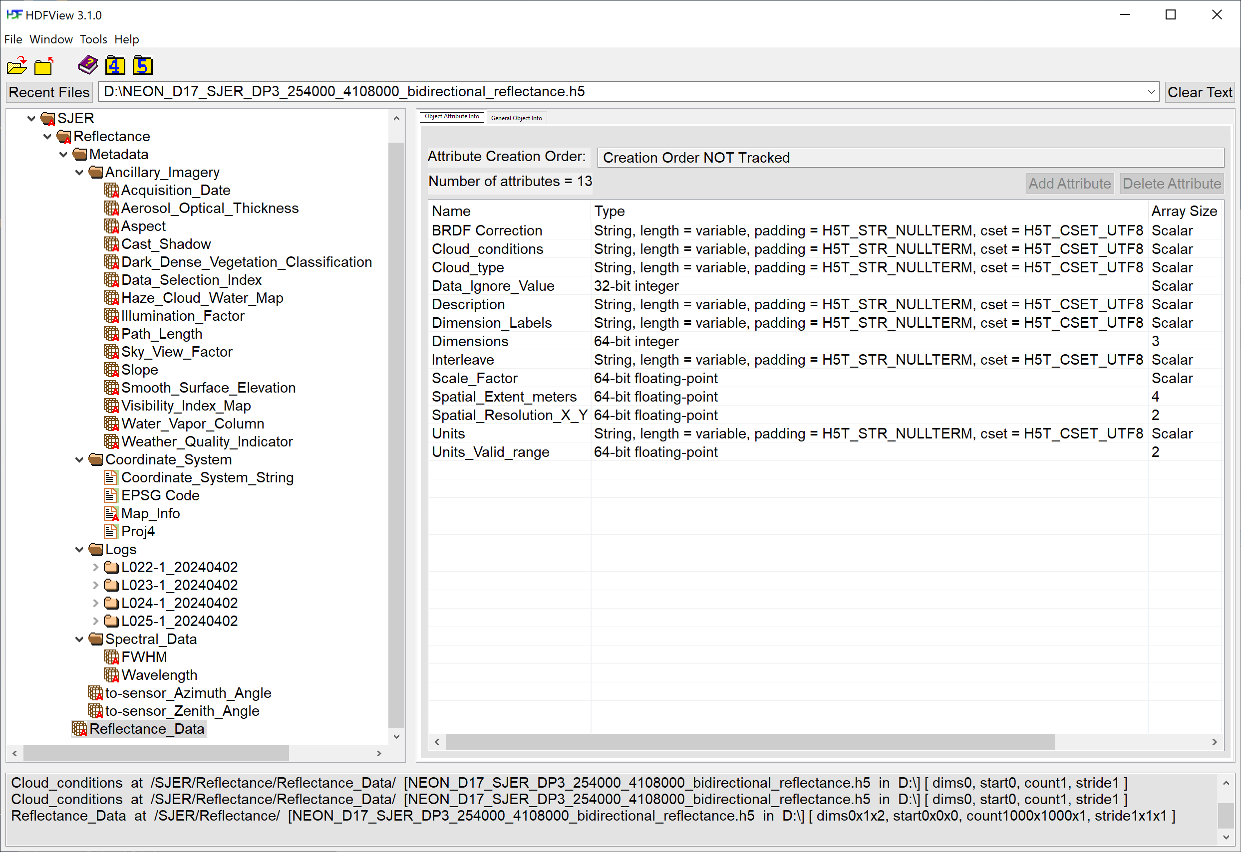
HDFView for a bidirectional reflectance hdf5 file for SJER
Open the Reflectance H5 file in HDFView
To begin, open the HDFView application.
Within the HDFView application, select File --> Open and navigate to the folder
where you saved the NEON_D17_SJER_DP3_254000_4108000_bidirectional_reflectance.h5 file on your computer. Open this file in HDFView.
Open the file and expand the sub-folders. This file is composed of a Reflectance dataset (called Reflectance_Data) along with additional Metadata containing the following sub-folders:
Ancillary_Imagery: Datasets including ATCOR inputs and other Quality indicators such as the Weather_Quality_Indicator, containing information about the cloud conditions during the flight (for each pixel).
Coordinate_System: geographic information for the dataset.
Logs: Log files for each flight line containing ATCOR processing information and inputs, BRDF correction parameters, and the solar azimuth and zenith angles.
Spectral_Data: Full Width Half Max (FWHM) and Wavelength for each of the 426 spectral bands.
Let's first look at the metadata stored in the Coordinate_System folder. This group
contains all of the spatial information that a GIS program would need to project
the data spatially.
Next, double click on the Wavelength dataset. Note that this dataset contains
the central wavelength value for each band in the dataset.
Finally, click on the Reflectance_Data dataset. Note that in the metadata for the
dataset that the structure of the dataset is 426 x 1000 x 1000 (wavelength, x,
y), as indicated in the metadata. Right click on the reflectance dataset
and select Open As. Click Image in the "display as" settings on the left hand
side of the popup.
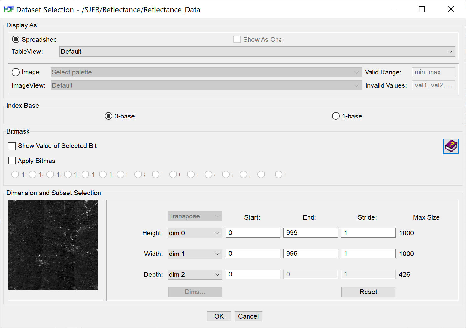
HDFView Reflectance Dataset Selection
Notice an image preview appears on the left of the pop-up window. Click OK to open
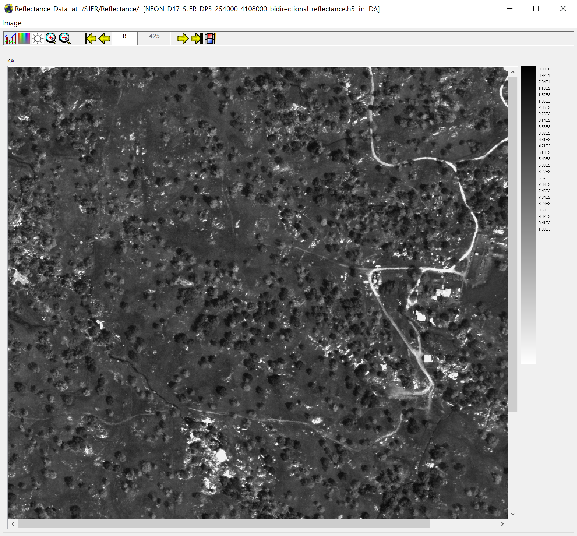
the image. You may have to play with the brightness and contrast settings in the
viewer to see the data properly.
HDFView Reflectance Preview
Explore the spectral dataset in the HDFViewer taking note of the metadata and data stored within the file.
Part 2: Exploring Surface Atmosphere Exchange (SAE) Data in HDFView
Next, we will look at the SAE bundled eddy covariance h5 data. As in the first part, we will start by opening the h5 file (download from the link at the top of this tutorial) in the viewer to get a better idea of how this data is structured.
Open the Bundled Eddy Covariance H5 file in HDFView
Open the HDFView application. Within the application, select File --> Open and navigate to the folder
where you saved the SAE hdf5 file on your computer. Open this file in HDFView.
If you click on the name of the HDF5 file in the left hand window of HDFView,
you can view metadata for the file. This will be located in the bottom window of
the application.
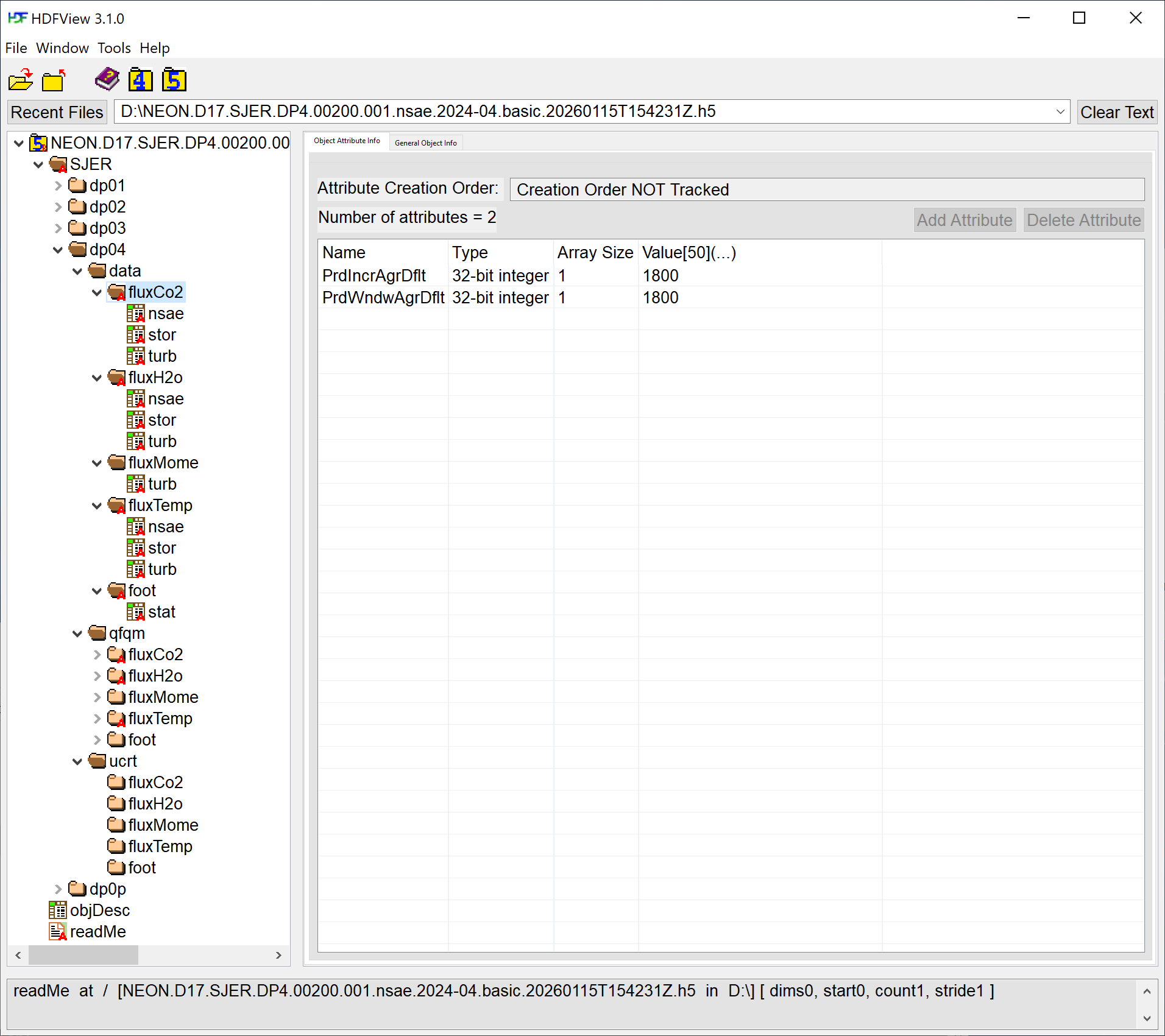
HDFView Reflectance Dataset Selection
Explore File Structure in HDFView
Next, explore the structure of this bundled eddy covariane file.
Notice at the bottom there is a readMe attribute. If you double click on this, you'll see the text "Net Surface Atmosphere Exchange (NSAE) HDF5 File Structure Description. The NSAE file you downloaded from NEON data portal is in the HDF5 format. This document describes the HDF5 file structure. This file will provide the HDF5 hierarchical layout of the file and a description of each HDF5 group level. The full descriptions of objects can be found in the objDesc data table provided within the HDF5 file. The 'Exploring NEON Eddy-Covariance Data Products in HDF5 file format' document provides a greater level of detail ..."
Documentation for each NEON data product is contained on the respective data product page. It is strongly recommended to peruse the relevant documentation, starting with the Quick Start Guides. The document referenced above in the readMe is linked here: Exploring NEON Eddy-Covariance Data Products in HDF5 file format .
Now that you've read the readMe, and referencing the document above, take a look at the structure of the data in HDFView.
Notice that there are multiple groups (folders) under the SJER root folder starting with dp. Expand these folders by double clicking on the folder icons. These represent the different data product levels, from 01 to 04, as well as level 0 prime.
dp01: Level 1
dp02: Level 2
dp03: Level 3
dp04: Level 4
dp0p: Level 0 prime
Under each of the levels there is a data folder with subfolders labeled by the data product identification codes as well as quality information (qfqm) and uncertainty (ucrt). Notice that there is also metadata associated with each group.
Within the dp04/data group there are five more groups: fluxCo2, fluxH2o, fluxMome, fluxTemp, and foot. What data are contained within these groups?
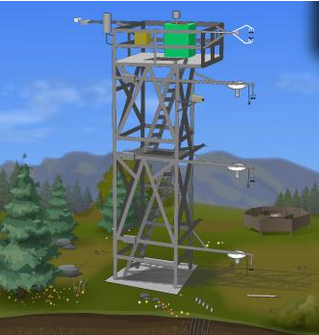
**Note:** The data used in this activity were collected by sensors mounted on a National Ecological Observatory Network (NEON) flux tower.
Read more about NEON towers here.
A NEON flux tower contains booms or arms that house sensors at varying heights along the tower.
So this is another example of how a NEON HDF5 file is structured. Take some time to explore this HDF5 dataset within the HDFViewer, using the reference document as needed.
Consider reviewing the documentation for the RHDF5 package.
A Brief Review - About HDF5
The HDF5 file can store large, heterogeneous datasets that include metadata. It
also supports efficient data slicing, or extraction of particular subsets of a
dataset which means that you don't have to read large files read into the computers
memory/RAM in their entirety in order work with them. This saves a lot of time
when working with with HDF5 data in R. When HDF5 files contain spatial data,
they can also be read directly into GIS programs such as QGiS.
The HDF5 format is a self-contained directory structure. We can compare this
structure to the folders and files located on your computer. However, in HDF5
files "directories" are called groups and files are called datasets. The
HDF5 element itself is a file. Each element in an HDF5 file can have metadata
attached to it making HDF5 files "self-describing".
The package we'll be using is rhdf5 which is part of the
Bioconductor suite of
R packages. If you haven't installed this package before, you can use the first
two lines of code below to install the package. Then use the library command to
call the library("rhdf5") library.
# Install rhdf5 package (only need to run if not already installed)
#install.packages("BiocManager")
#BiocManager::install("rhdf5")

# Call the R HDF5 Library
library("rhdf5")

# set working directory to ensure R can find the file we wish to import and where
# we want to save our files
wd <- "~/Documents/data/" #This will depend on your local environment
setwd(wd)
Let's start by outlining the structure of the file that we want to create.
We'll build a file called "sensorData.h5", that will hold data for a set of
sensors at three different locations. Each sensor takes three replicates of two
different measurements, every minute.
HDF5 allows us to organize and store data in many ways. Therefore we need to decide
what type of structure is ideally suited to our data before creating the HDF5 file.
To structure the HDF5 file, we'll start at the file level. We will create a group
for each sensor location. Within each location group, we will create two datasets
containing temperature and precipitation data collected through time at each location.
So it will look something like this:
HDF5 FILE (sensorData.H5)
Location_One (Group)
Temperature (Dataset)
Precipitation (Dataset)
Location_Two (Group)
Temperature (Dataset)
Precipitation (Dataset)
Location_Three (Group)
Temperature (Dataset)
Precipitation (Dataset)
Let's first create the HDF5 file and call it "sensorData.h5". Next, we will add
a group for each location to the file.
# create hdf5 file
h5createFile("sensorData.h5")

## file '/Users/olearyd/Git/data/sensorData.h5' already exists.

## [1] FALSE

# create group for location 1
h5createGroup("sensorData.h5", "location1")

## Can not create group. Object with name 'location1' already exists.

## [1] FALSE
The output is TRUE when the code properly runs.
Remember from the discussion above that we want to create three location groups. The
process of creating nested groups can be simplified with loops and nested loops.
While the for loop below might seem excessive for adding three groups, it will
become increasingly more efficient as we need to add more groups to our file.
# Create loops that will populate 2 additional location "groups" in our HDF5 file
	l1 <- c("location2","location3")
	for(i in 1:length(l1)){
  	  h5createGroup("sensorData.h5", l1[i])
	}

## Can not create group. Object with name 'location2' already exists.

## Can not create group. Object with name 'location3' already exists.
Now let's view the structure of our HDF5 file. We'll use the h5ls() function to do this.
# View HDF5 File Structure
h5ls("sensorData.h5")

##        group      name       otype dclass     dim
## 0          / location1   H5I_GROUP
## 1 /location1    precip H5I_DATASET  FLOAT 100 x 3
## 2 /location1      temp H5I_DATASET  FLOAT 100 x 3
## 3          / location2   H5I_GROUP
## 4 /location2    precip H5I_DATASET  FLOAT 100 x 3
## 5 /location2      temp H5I_DATASET  FLOAT 100 x 3
## 6          / location3   H5I_GROUP
## 7 /location3    precip H5I_DATASET  FLOAT 100 x 3
## 8 /location3      temp H5I_DATASET  FLOAT 100 x 3
Our group structure that will contain location information is now set-up. However,
it doesn't contain any data. Let's simulate some data pretending that each sensor
took replicate measurements for 100 minutes. We'll add a 100 x 3 matrix that will
be stored as a dataset in our HDF5 file. We'll populate this dataset with
simulated data for each of our groups. We'll use loops to create these matrices
and then paste them into each location group within the HDF5 file as datasets.
# Add datasets to each group
for(i in 1:3){
      g <- paste("location",i,sep="")

      # populate matrix with dummy data
      # create precip dataset within each location group
      h5write(
      	matrix(rnorm(300,2,1),
      				 ncol=3,nrow=100),
			file = "sensorData.h5",
			paste(g,"precip",sep="/"))

      #create temperature dataset within each location group
      h5write(
      	matrix(rnorm(300,25,5),
      				 ncol=3,nrow=100),
			file = "sensorData.h5",
			paste(g,"temp",sep="/"))
	}
Understandig Complex Code
Sometimes you may run into code (like the above code) that combines multiple
functions. It can be helpful to break the pieces of the code apart to understand
their overall function.
Looking at the first h5write() chunck above, let's figure out what it is doing.
We can see easily that part of it is telling R to create a matrix (matrix())
that has 3 columns (ncol=3) and 100 rows (nrow=100). That is fairly straight
forward, but what about the rest?
Do the following to figure out what it's doing.
Type paste(g,"precip",sep="/") into the R console. What is the result?
Type rnorm(300,2,1) into the console and see the result.
Type g into the console and take note of the result.
The rnorm function creates a set of random numbers that fall into a normal
distribution. You specify the mean and standard deviation of the dataset and R
does the rest. Notice in this loop we are creating a "precip" and a "temp" dataset
and pasting them into each location group (the loop iterates 3 times).
The h5write function is writing each matrix to a dataset in our HDF5 file
(sensorData.h5). It is looking for the following arguments: hrwrite(dataset,YourHdfFileName,LocationOfDatasetInH5File). Therefore, the code:
(matrix(rnorm(300,2,1),ncol=3,nrow=100),file = "sensorData.h5",paste(g,"precip",sep="/"))
tells R to add a random matrix of values to the sensorData HDF5 file within the
path called g. It also tells R to call the dataset within that group, "precip".
HDF5 File Structure
Next, let's check the file structure of the sensorData.h5 file. The h5ls()
command tells us what each element in the file is, group or dataset. It also
identifies the dimensions and types of data stored within the datasets in the
HDF5 file. In this case, the precipitation and temperature datasets are of type
'float' and of dimensions 100 x 3 (100 rows by 3 columns).
	# List file structure
	h5ls("sensorData.h5")

##        group      name       otype dclass     dim
## 0          / location1   H5I_GROUP
## 1 /location1    precip H5I_DATASET  FLOAT 100 x 3
## 2 /location1      temp H5I_DATASET  FLOAT 100 x 3
## 3          / location2   H5I_GROUP
## 4 /location2    precip H5I_DATASET  FLOAT 100 x 3
## 5 /location2      temp H5I_DATASET  FLOAT 100 x 3
## 6          / location3   H5I_GROUP
## 7 /location3    precip H5I_DATASET  FLOAT 100 x 3
## 8 /location3      temp H5I_DATASET  FLOAT 100 x 3
Data Types within HDF5
HDF5 files can hold mixed types of data. For example HDF5 files can store both
strings and numbers in the same file. Each dataset in an HDF5 file can be its
own type. For example a dataset can be composed of all integer values or it
could be composed of all strings (characters). A group can contain a mix of string,
and number based datasets. However a dataset can also be mixed within the dataset
containing a combination of numbers and strings.
Add Metdata to HDF5 Files
Some metadata can be added to an HDF5 file in R by creating attributes in R
objects before adding them to the HDF5 file. Let's look at an example of how we
do this. We'll add the units of our data as an attribute of the R matrix before
adding it to the HDF5 file. Note that write.attributes = TRUE is needed when
you write to the HDF5 file, in order to add metadata to the dataset.
# Create matrix of "dummy" data
p1 <- matrix(rnorm(300,2,1),ncol=3,nrow=100)
# Add attribute to the matrix (units)
attr(p1,"units") <- "millimeters"

# Write the R matrix to the HDF5 file
h5write(p1,file = "sensorData.h5","location1/precip",write.attributes=T)

# Close the HDF5 file
H5close()
We close the file at the end once we are done with it. Otherwise, next time you
open a HDF5 file, you will get a warning message similar to:
Warning message: In h5checktypeOrOpenLoc(file, readonly = TRUE) : An open HDF5 file handle exists. If the file has changed on disk meanwhile, the function may not work properly. Run 'H5close()' to close all open HDF5 object handles.
Reading Data from an HDF5 File
We just learned how to create an HDF5 file and write information to the file.
We use a different set of functions to read data from an HDF5 file. If
read.attributes is set to TRUE when we read the data, then we can also see
the metadata for the matrix. Furthermore, we can chose to read in a subset,
like the first 10 rows of data, rather than loading the entire dataset into R.
# Read in all data contained in the precipitation dataset
l1p1 <- h5read("sensorData.h5","location1/precip",
							 read.attributes=T)

# Read in first 10 lines of the data contained within the precipitation dataset
l1p1s <- h5read("sensorData.h5","location1/precip",
								read.attributes = T,index = list(1:10,NULL))
Now you are ready to go onto the other tutorials in the series to explore more
about HDF5 files.
### Challenge: Your Own HDF5
Think about an application for HDF5 that you might have. Create a new HDF5 file
that would support the data that you need to store.
### Challenge: View Data with HDFView
Open the sensordata.H5 file in the HDFView application and explore the contents.
R is a versatile, open source programming language that was specifically
designed for data analysis. R is extremely useful for data management,
statistics and analyzing data.
This tutorial should be seem more as a reference on the basics of R and not a
tutorial for learning to use R. Here we define many of the basics, however, this
can get overwhelming if you are brand new to R.
Learning Objectives
After completing this tutorial, you will be able to:
Use basic R syntax
Explain the concepts of objects and assignment
Explain the concepts of vector and data types
Describe why you would or would not use factors
Use basic few functions
Things You’ll Need To Complete This Tutorial
You will need the most current version of R and, preferably, RStudio loaded
on your computer to complete this tutorial.
Set Working Directory: This lesson assumes that you have set your working
directory to the location of the downloaded and unzipped data subsets.
R Script & Challenge Code: NEON data lessons often contain challenges that
reinforce learned skills. If available, the code for challenge solutions is
found in the downloadable R script of the entire lesson, available in the footer
of each lesson page.
The Very Basics of R
R is a versatile, open source programming language that was specifically
designed for data analysis. R is extremely useful for data management,
statistics and analyzing data.
**Cool Fact:** R was inspired by the programming language S.
A good alternative to commercial analysis tools. R has over 5,000 user
contributed packages (as of 2014) and is widely used both in academia and
industry.
Available on all platforms.
Not just for statistics, but also general purpose programming.
Supported by a large and growing community of peers.
Introduction to R
You can use R alone or with a user interace like RStudio to write your code.
Some people prefer RStudio as it provides a graphic interface where you can see
what objects have been created and you can also set variables like your working
directory, using menu options.
We want to use R to create code and a workflow is more reproducible. We can
document everything that we do. Our end goal is not just to "do stuff" but to
do it in a way that anyone can easily and exactly replicate our workflow and
results -- this includes ourselves in 3 months when the paper reviews come back!
Code & Comments in R
Everything you type into an R script is code, unless you demark it otherwise.
Anything to the right of a # is ignored by R. Use these comments within the
code to describe what it is that you code is doing. Comment liberally in your R
scripts. This will help you when you return to it and will also help others
understand your scripts and analyses.
# this is a comment. It allows text that is ignored by the program.
# for clean, easy to read comments, use a space between the # and text.

# there is a line of code below this comment
 a <- 1 + 2
Basic Operations in R
Let's take a few moments to play with R. You can get output from R simply by
typing in math
or by typing words, with the command writeLines(). Words that you want to be
recognized as text (as opposed to a field name or other text that signifies an
object) must be enclosed within quotes.
# have R write words

writeLines("Hello World")

## Hello World
We can assign our results to an object and name the object. Objects names
cannot contain spaces.
# assigning values to objects
secondsPerHour <- 60 * 60

hoursPerYear <- 365 * 24


# object names can't contain spaces.  Use a period, underscore, or camelCase to
# create longer names
temp_HARV <- 90
par.OSBS <- 180
We can then return the value of an object we created.
The result of the operation on the right hand side of <- is assigned to
an object with the name specified on the left hand side of <-. The result
could be any type of R object, including your own functions (see the
Build & Work With Functions in R tutorial).
Assignment Operator: Drop the Equals Sign
The assignment operator is <-. It assigns values on the right to objects on
the left. It is similar to = but there are some subtle differences. Learn to
use <- as it is good programming practice. Using = in place of <- can lead
to issues down the line.
# this is preferred syntax
a <- 1 + 2

# this is NOT preferred syntax
a = 1 + 2
**Typing Tip:** If you are using RStudio, you can use
a keyboard shortcut for the assignment operator: **Windows/Linux: "Alt" + "-"**
or **Mac: "Option" + "-"**.
List All Objects in the Environment
Some functions are the same as in other languages. These might be familiar from
command line.
ls(): to list objects in your current environment.
rm(): remove objects from your current environment.
Now try them in the console.
# assign value "5" to object "x"
x <- 5
ls()

# remove x
rm(x)

# what is left?
ls()

# remove all objects
rm(list = ls())

ls()
Using rm(list=ls()), you combine several functions to remove all objects.
If you typed x on the console now you will get Error: object 'x' not found'.
Data Types and Structures
To make the best of the R language, you'll need a strong understanding of the
basic data types and data structures and how to operate on those. These are the
objects you will manipulate on a day-to-day basis in R. Dealing with object
conversions is one of the most common sources of frustration for beginners.
First, everything in R is an object. But there are different types of
objects. One of the basic differences in in the data structures which are
different ways data are stored.
R has many different data structures. These include
atomic vector
list
matrix
data frame
array
These data structures vary by the dimensionality of the data and if they can
handle data elements of a simgle type (homogeneous) or multiple types
(heterogeneous).
Dimensions
Homogenous
Heterogeneous
1-D
atomic vector
list
2-D
matrix
data frame
none
array
Vectors
A vector is the most common and basic data structure in R and is the workhorse
of R. Technically, vectors can be one of two types:
atomic vectors
lists
although the term "vector" most commonly refers to the atomic types not to lists.
Atomic Vectors
R has 6 atomic vector types.
character
numeric (real or decimal)
integer
logical
complex
raw (not discussed in this tutorial)
By atomic, we mean the vector only holds data of a single type.
character: "a", "swc"
numeric: 2, 15.5
integer: 2L (the L tells R to store this as an integer)
logical: TRUE, FALSE
complex: 1+4i (complex numbers with real and imaginary parts)
R provides many functions to examine features of vectors and other objects, for
example
typeof() - what is it?
length() - how long is it? What about two dimensional objects?
attributes() - does it have any metadata?
Let's look at some examples:
# assign word "april" to x"
x <- "april"

# return the type of the object
class(x)

## [1] "character"

# does x have any attributes?
attributes(x)

## NULL

# assign all integers 1 to 10 as an atomic vector to the object y
y <- 1:10
y

##  [1]  1  2  3  4  5  6  7  8  9 10

class(y)

## [1] "integer"

# how many values does the vector y contain?
length(y)

## [1] 10

# coerce the integer vector y to a numeric vector
# store the result in the object z
z <- as.numeric(y)
z

##  [1]  1  2  3  4  5  6  7  8  9 10

class(z)

## [1] "numeric"
A vector is a collection of elements that are most commonly character,
logical, integer or numeric.
You can create an empty vector with vector(). (By default the mode is
logical. You can be more explicit as shown in the examples below.) It is more
common to use direct constructors such as character(), numeric(), etc.
x <- vector()

# Create vector with a length and type
vector("character", length = 10)

##  [1] "" "" "" "" "" "" "" "" "" ""

# create character vector with length of 5
character(5)

## [1] "" "" "" "" ""

# numeric vector length=5
numeric(5)

## [1] 0 0 0 0 0

# logical vector length=5
logical(5)

## [1] FALSE FALSE FALSE FALSE FALSE

# create a list or vector with combine `c()`
# this is the function used to create vectors and lists most of the time
x <- c(1, 2, 3)
x

## [1] 1 2 3

length(x)

## [1] 3

class(x)

## [1] "numeric"
x is a numeric vector. These are the most common kind. They are numeric
objects and are treated as double precision real numbers (they can store
decimal points). To explicitly create integers (no decimal points), add an
L to each (or coerce to the integer type using as.integer().
# a numeric vector with integers (L)
x1 <- c(1L, 2L, 3L)
x1

## [1] 1 2 3

class(x1)

## [1] "integer"

# or using as.integer()
x2 <- as.integer(x)
class(x2)

## [1] "integer"
You can also have logical vectors.
# logical vector
y <- c(TRUE, TRUE, FALSE, FALSE)
y

## [1]  TRUE  TRUE FALSE FALSE

class(y)

## [1] "logical"
Finally, you can have character vectors.
# character vector
z <- c("Sarah", "Tracy", "Jon")
z

## [1] "Sarah" "Tracy" "Jon"

# what class is it?
class(z)

## [1] "character"

#how many elements does it contain?
length(z)

## [1] 3

# what is the structure?
str(z)

##  chr [1:3] "Sarah" "Tracy" "Jon"
You can also add to a list or vector
# c function combines z and "Annette" into a single vector
# store result back to z
z <- c(z, "Annette")
z

## [1] "Sarah"   "Tracy"   "Jon"     "Annette"
More examples of how to create vectors
x <- c(0.5, 0.7)
x <- c(TRUE, FALSE)
x <- c("a", "b", "c", "d", "e")
x <- 9:100
x <- c(1 + (0 + 0i), 2 + (0 + 4i))
You can also create vectors as a sequence of numbers.
Inf is infinity. You can have either positive or negative infinity.
NaN means Not a Number. It's an undefined value.
Try it out in the console.
# infinity return
1/0

## [1] Inf

# non numeric return
0/0

## [1] NaN
Indexing
Vectors have positions, these positions are ordered and can be called using
object[index]
# index
z[2]

## [1] "Tracy"

# to call multiple items (a subset of our data), we can put a vector of which
# items we want in the brackets
group1 <- c(1, 4)
z[group1]

## [1] "Sarah"   "Annette"

# this is especially useful with a sequence vector
z[1:3]

## [1] "Sarah" "Tracy" "Jon"
Objects can have attributes. Attribues are part of the object. These
include:
names: the field or variable name within the object
dimnames:
dim:
class:
attributes: this contain metadata
You can also glean other attribute-like information such as length()
(works on vectors and lists) or number of characters nchar() (for
character strings).
# length of an object
length(1:10)

## [1] 10

length(x)

## [1] 3

# number of characters in a text string
nchar("NEON Data Skills")

## [1] 16
Heterogeneous Data - Mixing Types?
When you mix types, R will create a resulting vector that is the least common
denominator. The coercion will move towards the one that's easiest to coerce
to.
Guess what the following do:
m <- c(1.7, "a")
n <- c(TRUE, 2)
o <- c("a", TRUE)
Were you correct?
n <- c(1.7, "a")
n

## [1] "1.7" "a"

o <- c(TRUE, 2)
o

## [1] 1 2

p <- c("a", TRUE)
p

## [1] "a"    "TRUE"
This is called implicit coercion. You can also coerce vectors explicitly using
the as.<class_name>.
# making values numeric
as.numeric("1")

## [1] 1

# make values charactor
as.character(1)

## [1] "1"

# make values
as.factor(c("male", "female"))

## [1] male   female
## Levels: female male
Matrix
In R, matrices are an extension of the numeric or character vectors. They are
not a separate type of object but simply an atomic vector with dimensions; the
number of rows and columns.
# create an empty matrix that is 2x2
m <- matrix(nrow = 2, ncol = 2)
m

##      [,1] [,2]
## [1,]   NA   NA
## [2,]   NA   NA

# what are the dimensions of m
dim(m)

## [1] 2 2
Matrices in R are by default filled column-wise. You can also use the byrow
argument to specify how the matrix is filled.
# create a matrix. Notice R fills them by columns by default
m2 <- matrix(1:6, nrow = 2, ncol = 3)
m2

##      [,1] [,2] [,3]
## [1,]    1    3    5
## [2,]    2    4    6

# set the byrow argument to TRUE to fill by rows
m2_row <- matrix(c(1:6), nrow = 2, ncol = 3, byrow = TRUE)
m2_row

##      [,1] [,2] [,3]
## [1,]    1    2    3
## [2,]    4    5    6
dim() takes a vector and transform into a matrix with 2 rows and 5 columns.
Another way to shape your matrix is to bind columns cbind() or rows rbind().
# create vector with 1:10
m3 <- 1:10
m3

##  [1]  1  2  3  4  5  6  7  8  9 10

class(m3)

## [1] "integer"

# set the dimensions so it becomes a matrix
dim(m3) <- c(2, 5)
m3

##      [,1] [,2] [,3] [,4] [,5]
## [1,]    1    3    5    7    9
## [2,]    2    4    6    8   10

class(m3)

## [1] "matrix" "array"

# create matrix from two vectors
x <- 1:3
y <- 10:12

# cbind will bind the two by column
cbind(x, y)

##      x  y
## [1,] 1 10
## [2,] 2 11
## [3,] 3 12

# rbind will bind the two by row
rbind(x, y)

##   [,1] [,2] [,3]
## x    1    2    3
## y   10   11   12
Matrix Indexing
We can call elements of a matrix with square brackets just like a vector, except
now we must specify a row and a column.
z <- matrix(c("a", "b", "c", "d", "e", "f"), nrow = 3, ncol = 2)
z

##      [,1] [,2]
## [1,] "a"  "d"
## [2,] "b"  "e"
## [3,] "c"  "f"

# call element in the third row, second column
z[3, 2]

## [1] "f"

# leaving the row blank will return contents of the whole column
# note: the column's contents are displayed as a vector (horizontally)
z[, 2]

## [1] "d" "e" "f"

class(z[, 2])

## [1] "character"

# return the contents of the second row
z[2, ]

## [1] "b" "e"
List
In R, lists act as containers. Unlike atomic vectors, the contents of a list are
not restricted to a single mode and can encompass any mixture of data types.
Lists are sometimes called generic vectors, because the elements of a list can
by of any type of R object, even lists containing further lists. This property
makes them fundamentally different from atomic vectors.
A list is different from an atomic vector because each element can be a
different type -- it can contain heterogeneous data types.
Create lists using list() or coerce other objects using as.list(). An empty
list of the required length can be created using vector()
x <- list(1, "a", TRUE, 1 + (0 + 4i))
x

## [[1]]
## [1] 1
##
## [[2]]
## [1] "a"
##
## [[3]]
## [1] TRUE
##
## [[4]]
## [1] 1+4i

class(x)

## [1] "list"

x <- vector("list", length = 5)  ## empty list
length(x)

## [1] 5

#call the 1st element of list x
x[[1]]

## NULL

x <- 1:10
x <- as.list(x)
Questions:
What is the class of x[1]?
What about x[[1]]?
Try it out.
We can also give the elements of our list names, then call those elements with
the $ operator.
# note 'iris' is an example data frame included with R
# the head() function simply calls the first 6 rows of the data frame
xlist <- list(a = "Karthik Ram", b = 1:10, data = head(iris))
xlist

## $a
## [1] "Karthik Ram"
##
## $b
##  [1]  1  2  3  4  5  6  7  8  9 10
##
## $data
##   Sepal.Length Sepal.Width Petal.Length Petal.Width Species
## 1          5.1         3.5          1.4         0.2  setosa
## 2          4.9         3.0          1.4         0.2  setosa
## 3          4.7         3.2          1.3         0.2  setosa
## 4          4.6         3.1          1.5         0.2  setosa
## 5          5.0         3.6          1.4         0.2  setosa
## 6          5.4         3.9          1.7         0.4  setosa

# see names of our list elements
names(xlist)

## [1] "a"    "b"    "data"

# call individual elements by name
xlist$a

## [1] "Karthik Ram"

xlist$b

##  [1]  1  2  3  4  5  6  7  8  9 10

xlist$data

##   Sepal.Length Sepal.Width Petal.Length Petal.Width Species
## 1          5.1         3.5          1.4         0.2  setosa
## 2          4.9         3.0          1.4         0.2  setosa
## 3          4.7         3.2          1.3         0.2  setosa
## 4          4.6         3.1          1.5         0.2  setosa
## 5          5.0         3.6          1.4         0.2  setosa
## 6          5.4         3.9          1.7         0.4  setosa
What is the length of this object? What about its structure?
Lists can be extremely useful inside functions. You can “staple” together
lots of different kinds of results into a single object that a function can
return.
A list does not print to the console like a vector. Instead, each element
of the list starts on a new line.
Elements are indexed by double brackets. Single brackets will still return
a(nother) list.
Factors
Factors are special vectors that represent categorical data. Factors can be
ordered or unordered and are important for modelling functions such as lm()
and glm() and also in plot() methods. Once created, factors can only contain
a pre-defined set values, known as levels.
Factors are stored as integers that have labels associated the unique integers.
While factors look (and often behave) like character vectors, they are actually
integers under the hood. You need to be careful when treating them like strings.
Some string methods will coerce factors to strings, while others will throw an
error.
Sometimes factors can be left unordered. Example: male, female.
Other times you might want factors to be ordered (or ranked). Example: low,
medium, high.
Underlying it's represented by numbers 1, 2, 3.
They are better than using simple integer labels because factors are what are
called self describing. male and female is more descriptive than 1s and 2s.
Helpful when there is no additional metadata.
Which is male? 1 or 2? You wouldn't be able to tell with just integer data.
Factors have this information built in.
Factors can be created with factor(). Input is often a character vector.
x <- factor(c("yes", "no", "no", "yes", "yes"))
x

## [1] yes no  no  yes yes
## Levels: no yes
table(x) will return a frequency table counting the number of elements in
each level.
If you need to convert a factor to a character vector, simply use
To see the integer version of the factor levels, use as.numeric
as.numeric(x)

## [1] 2 1 1 2 2
To convert a factor to a numeric vector, go via a character. Compare
fac <- factor(c(1, 5, 5, 10, 2, 2, 2))

levels(fac)       ## returns just the four levels present in our factor

## [1] "1"  "2"  "5"  "10"

as.numeric(fac)   ## wrong! returns the assigned integer for each level

## [1] 1 3 3 4 2 2 2

                ## integer corresponds to the position of that number in levels(f)

as.character(fac) ## returns a character string of each number

## [1] "1"  "5"  "5"  "10" "2"  "2"  "2"

as.numeric(as.character(fac)) ## coerce the character strings to numbers

## [1]  1  5  5 10  2  2  2
In modeling functions, it is important to know what the 'baseline' level is. This
is the first factor, but by default the ordering is determined by alphanumerical
order of elements. You can change this by speciying the levels (another option
is to use the function relevel()).
# the default result (because N comes before Y alphabetically)
x <- factor(c("yes", "no", "yes"))
x

## [1] yes no  yes
## Levels: no yes

# now let's try again, this time specifying the order of our levels
x <- factor(c("yes", "no", "yes"), levels = c("yes", "no"))
x

## [1] yes no  yes
## Levels: yes no
Data Frames
A data frame is a very important data type in R. It's pretty much the de facto
data structure for most tabular data and what we use for statistics.
A data frame is a special type of list where every element of the list has
same length.
Data frames can have additional attributes such as rownames(), which can
be useful for annotating data, like subject_id or sample_id. But most of
the time they are not used.
Some additional information on data frames:
Usually created by read.csv() and read.table().
Can convert to matrix with data.matrix() (preferred) or as.matrix()
Coercion will be forced and not always what you expect.
Can also create with data.frame() function.
Find the number of rows and columns with nrow(dat) and ncol(dat),
respectively.
Rownames are usually 1, 2, ..., n.
Manually Create Data Frames
You can manually create a data frame using data.frame.
# create a dataframe
dat <- data.frame(id = letters[1:10], x = 1:10, y = 11:20)
dat

##    id  x  y
## 1   a  1 11
## 2   b  2 12
## 3   c  3 13
## 4   d  4 14
## 5   e  5 15
## 6   f  6 16
## 7   g  7 17
## 8   h  8 18
## 9   i  9 19
## 10  j 10 20
Useful Data Frame Functions
head() - shown first 6 rows
tail() - show last 6 rows
dim() - returns the dimensions
nrow() - number of rows
ncol() - number of columns
str() - structure of each column
names() - shows the names attribute for a data frame, which gives the
column names.
Instead of a list of single items, a data frame is a list of vectors!
# see the class of a single variable column within iris: "Sepal.Length"
class(iris$Sepal.Length)

## [1] "numeric"
A recap of the different data types
Dimensions
Homogenous
Heterogeneous
1-D
atomic vector
list
2-D
matrix
data frame
none
array
Functions
A function is an R object that takes inputs to perform a task.
Functions take in information and may return desired outputs.
output <- name_of_function(inputs)
# create a list of 1 to 10
x <- 1:10

# the sum of all x
y <- sum(x)
y

## [1] 55
Help
All functions come with a help screen. It is critical that you learn to read the
help screens since they provide important information on what the function does,
how it works, and usually sample examples at the very bottom. You can use
help(function) or more simply ??function
# call up a help search
help.start()

# help (documentation) for a package
??ggplot2

# help for a function
??sum()
You can't ever learn all of R as it is ever changing with new packages and new
tools, but once you have the basics and know how to find help to do the things
that you want to do, you'll be able to use R in your science.
Sample Data
R comes with sample datasets. You will often find these as the date sets in
documentation files or responses to inquires on public forums like StackOverflow.
To see all available sample datasets you can type in data() to the console.
Packages in R
R comes with a set of functions or commands that perform particular sets of
calculations. For example, in the equation 1+2, R knows that the "+" means to
add the two numbers, 1 and 2 together. However, you can expand the capability of
R by installing packages that contain suites of functions and compiled code that
you can also use in your code.
The LiDAR and imagery data used to create the rasters in this dataset were
collected over the San Joaquin field site located in California (NEON Domain 17)
and processed at NEON
headquarters. The entire dataset can be accessed by request from the NEON website.
This data download contains several files used in related tutorials. The path to
the files we will be using in this tutorial is:
NEON-DS-Field-Site-Spatial-Data/SJER/.
You should set your working directory to the parent directory of the downloaded
data to follow the code exactly.
This tutorial will overview the key attributes of a raster object, including
spatial extent, resolution and coordinate reference system. When working within
a GIS system often these attributes are accounted for. However, it is important
to be more familiar with them when working in non-GUI environments such as
R or even Python.
In order to correctly spatially reference a raster that is not already georeferenced,
you will also need to identify:
The lower left hand corner coordinates of the raster.
The number of columns and rows that the raster dataset contains.
Spatial Resolution
A raster consists of a series of pixels, each with the same dimensions
and shape. In the case of rasters derived from airborne sensors, each pixel
represents an area of space on the Earth's surface. The size of the area on the
surface that each pixel covers is known as the spatial resolution of the image.
For instance, an image that has a 1 m spatial resolution means that each pixel in
the image represents a 1 m x 1 m area.
The spatial resolution of a raster refers the size of each cell
in meters. This size in turn relates to the area on the ground that the pixel
represents. Source: National Ecological Observatory Network (NEON) A raster at the same extent with more pixels will have a higher
resolution (it looks more "crisp"). A raster that is stretched over the same
extent with fewer pixels will look more blury and will be of lower resolution.
Source: National Ecological Observatory Network (NEON)
Load the Data
Let's open up a raster in R to see how the attributes are stored. We are
going to work with a Digital Terrain Model from the San Joaquin Experimental
Range in California.
# load packages
library(raster)
library(rgdal)

# set working directory to data folder
#setwd("pathToDirHere")
wd <- ("~/Git/data/")
setwd(wd)

# Load raster in an R object called 'DEM'
DEM <- raster(paste0(wd, "NEON-DS-Field-Site-Spatial-Data/SJER/DigitalTerrainModel/SJER2013_DTM.tif"))


# View raster attributes
DEM

## class      : RasterLayer
## dimensions : 5060, 4299, 21752940  (nrow, ncol, ncell)
## resolution : 1, 1  (x, y)
## extent     : 254570, 258869, 4107302, 4112362  (xmin, xmax, ymin, ymax)
## crs        : +proj=utm +zone=11 +datum=WGS84 +units=m +no_defs
## source     : /Users/olearyd/Git/data/NEON-DS-Field-Site-Spatial-Data/SJER/DigitalTerrainModel/SJER2013_DTM.tif
## names      : SJER2013_DTM
Note that this raster (in GeoTIFF format) already has an extent, resolution, and
CRS defined. The resolution in both x and y directions is 1. The CRS tells us
that the x,y units of the data are meters (m).
Spatial Extent
The spatial extent of a raster, represents the "X, Y" coordinates of the corners
of the raster in geographic space. This information, in addition to the cell
size or spatial resolution, tells the program how to place or render each pixel
in 2 dimensional space. Tools like R, using supporting packages such as rgdal
and associated raster tools have functions that allow you to view and define the
extent of a new raster.
# View the extent of the raster
DEM@extent

## class      : Extent
## xmin       : 254570
## xmax       : 258869
## ymin       : 4107302
## ymax       : 4112362
If you double the extent value of a raster - the pixels will be
stretched over the larger area making it look more "blury". Source: National
Ecological Observatory Network (NEON)
Calculating Raster Extent
Extent and spatial resolution are closely connected. To calculate the extent of a
raster, we first need the bottom left hand (X,Y) coordinate of the raster. In
the case of the UTM coordinate system which is in meters, to calculate
the raster's extent, we can add the number of columns and rows to the X,Y corner
coordinate location of the raster, multiplied by the resolution (the pixel size)
of the raster.
<figcaption>To be located geographically, a raster's location needs to be
defined in geographic space (i.e., on a spatial grid). The spatial extent
defines the four corners of a raster within a given coordinate reference
system. Source: National Ecological Observatory Network. </figcaption>
Let's explore that next, using a blank raster that we create.
# create a raster from the matrix - a "blank" raster of 4x4
myRaster1 <- raster(nrow=4, ncol=4)

# assign "data" to raster: 1 to n based on the number of cells in the raster
myRaster1[]<- 1:ncell(myRaster1)

# view attributes of the raster
myRaster1

## class      : RasterLayer
## dimensions : 4, 4, 16  (nrow, ncol, ncell)
## resolution : 90, 45  (x, y)
## extent     : -180, 180, -90, 90  (xmin, xmax, ymin, ymax)
## crs        : +proj=longlat +datum=WGS84 +no_defs
## source     : memory
## names      : layer
## values     : 1, 16  (min, max)

# is the CRS defined?
myRaster1@crs

## CRS arguments: +proj=longlat +datum=WGS84 +no_defs
Wait, why is the CRS defined on this new raster? This is the default values
for something created with the raster() function if nothing is defined.
Let's get back to looking at more attributes.
# what is the raster extent?
myRaster1@extent

## class      : Extent
## xmin       : -180
## xmax       : 180
## ymin       : -90
## ymax       : 90

# plot raster
plot(myRaster1, main="Raster with 16 pixels")
Here we see our raster with the value of 1 to 16 in each pixel.
We can resample the raster as well to adjust the resolution. If we want a higher
resolution raster, we will apply a grid with more pixels within the same extent.
If we want a lower resolution raster, we will apply a grid with fewer pixels
within the same extent.
One way to do this is to create a raster of the resolution you want and then
resample() your original raster. The resampling will be done for either
nearest neighbor assignments (for categorical data) or bilinear interpolation (for
numerical data).
To more easily compare them, let's create a graphic layout with 4 rasters in it.
Notice that each raster has the same extent but each a different resolution
because it has a different number of pixels spread out over the same extent.
# change graphical parameter to 2x2 grid
par(mfrow=c(2,2))

# arrange plots in order you wish to see them
plot(myRaster2, main="Raster with 32 pixels")
plot(myRaster1, main="Raster with 16 pixels")
plot(myRaster3, main="Raster with 4 pixels")
plot(myRaster4, main="Raster with 2 pixels")
# change graphical parameter back to 1x1
par(mfrow=c(1,1))
Extent & Coordinate Reference Systems
The X and Y min and max values relate to the coordinate system
that the file is in, see below.
Coordinate Reference System & Projection Information
A spatial reference system (SRS) or coordinate reference system (CRS) is a
coordinate-based local, regional or global system used to locate geographical
entities. -- Wikipedia
The earth is round. This is not an new concept by any means, however we need to
remember this when we talk about coordinate reference systems associated with
spatial data. When we make maps on paper or on a computer screen, we are moving
from a 3 dimensional space (the globe) to 2 dimensions (our computer screens or
a piece of paper). To keep this short, the projection of a dataset relates to
how the data are "flattened" in geographic space so our human eyes and brains
can make sense of the information in 2 dimensions.
The projection refers to the mathematical calculations performed to "flatten the
data" in into 2D space. The coordinate system references to the x and y coordinate
space that is associated with the projection used to flatten the data. If you
have the same dataset saved in two different projections, these two files won't
line up correctly when rendered together.
Maps of the United States in different projections. Notice the
differences in shape associated with each different projection. These
differences are a direct result of the calculations used to "flatten" the
data onto a 2 dimensional map. Source: M. Corey, opennews.org
Check out this short video,
by Buzzfeed, highlighting how map projections can make continents
seems proportionally larger or smaller than they actually are!
What Makes Spatial Data Line Up On A Map?
There are lots of great resources that describe coordinate reference systems and
projections in greater detail. However, for the purposes of this activity, what
is important to understand is that data from the same location but saved in
different projections will not line up in any GIS or other program. Thus
it's important when working with spatial data in a program like R or Python
to identify the coordinate reference system applied to the data, and to grab
that information and retain it when you process / analyze the data.
The rgdal package has all the common ESPG codes with proj4string built in. We
can see them by creating an object of the function make_ESPG().
# make sure you loaded rgdal package at the top of your script

# create an object with all ESPG codes
epsg = make_EPSG()

# use View(espg) to see the full table - doesn't render on website well
#View(epsg)

# View top 5 entries
head(epsg, 5)

##   code   note                                                   prj4
## 1 3819 HD1909         +proj=longlat +ellps=bessel +no_defs +type=crs
## 2 3821  TWD67        +proj=longlat +ellps=aust_SA +no_defs +type=crs
## 3 3822  TWD97 +proj=geocent +ellps=GRS80 +units=m +no_defs +type=crs
## 4 3823  TWD97          +proj=longlat +ellps=GRS80 +no_defs +type=crs
## 5 3824  TWD97          +proj=longlat +ellps=GRS80 +no_defs +type=crs
##   prj_method
## 1     (null)
## 2     (null)
## 3     (null)
## 4     (null)
## 5     (null)
Define the extent
In the above raster example, we created several simple raster objects in R.
R defaulted to a global lat/long extent. We can define the exact extent that we
need to use too.
Let's create a new raster with the same projection as our original DEM. We know
that our data are in UTM zone 11N. For the sake of this exercise, let say we
want to create a raster with the left hand corner coordinate at:
xmin = 254570
ymin = 4107302
The resolution of this new raster will be 1 meter and we will be working
in UTM (meters). First, let's set up the raster.
Now we can define the new raster's extent by defining the lower left corner of
the raster.
## Define the xmin and ymin (the lower left hand corner of the raster)

# 1. define xMin & yMin objects.
xMin = 254570
yMin = 4107302

# 2. grab the cols and rows for the raster using @ncols and @nrows
rasterNoProj@ncols

## [1] 20

rasterNoProj@nrows

## [1] 10

# 3. raster resolution
res <- 1.0

# 4. add the numbers of cols and rows to the x,y corner location,
# result = we get the bounds of our raster extent.
xMax <- xMin + (rasterNoProj@ncols * res)
yMax <- yMin + (rasterNoProj@nrows * res)

# 5.create a raster extent class
rasExt <- extent(xMin,xMax,yMin,yMax)
rasExt

## class      : Extent
## xmin       : 254570
## xmax       : 254590
## ymin       : 4107302
## ymax       : 4107312

# 6. apply the extent to our raster
rasterNoProj@extent <- rasExt

# Did it work?
rasterNoProj

## class      : RasterLayer
## dimensions : 10, 20, 200  (nrow, ncol, ncell)
## resolution : 1, 1  (x, y)
## extent     : 254570, 254590, 4107302, 4107312  (xmin, xmax, ymin, ymax)
## crs        : NA
## source     : memory
## names      : layer
## values     : 1, 8  (min, max)

# or view extent only
rasterNoProj@extent

## class      : Extent
## xmin       : 254570
## xmax       : 254590
## ymin       : 4107302
## ymax       : 4107312
Now we have an extent associated with our raster which places it in space!
# plot new raster
plot(rasterNoProj, main="Raster in UTM coordinates, 1 m resolution")
Notice that the coordinates show up on our plot now.
## Challenges: Resample Rasters
Now apply your skills in a new way!
Resample rasterNoProj from 1 meter to 10 meter resolution. Plot it next to the 1 m
resolution raster. Use: par(mfrow=c(1,2)) to create side by side plots.
What happens to the extent if you change the resolution to 1.5 when calculating
the raster's extent properties??
Define Projection of a Raster
We can define the projection of a raster that has a known CRS already. Sometimes
we download data that have projection information associated with them but the CRS
is not defined either in the GeoTIFF tags or in the raster itself. If this is the
case, we can simply assign the raster the correct projection.
Be careful doing this - it is not the same thing as reprojecting your data.
Let's define the projection for our newest raster using the DEM raster that
already has defined CRS. NOTE: in this case we have to know that our raster is
in this projection already so we don't run the risk of assigning the wrong projection
to the data.
# view CRS from raster of interest
rasterNoProj@crs

## CRS arguments: NA

# view the CRS of our DEM object.
DEM@crs

## CRS arguments:
##  +proj=utm +zone=11 +datum=WGS84 +units=m +no_defs

# define the CRS using a CRS of another raster
rasterNoProj@crs <- DEM@crs

# look at the attributes
rasterNoProj

## class      : RasterLayer
## dimensions : 10, 20, 200  (nrow, ncol, ncell)
## resolution : 1, 1  (x, y)
## extent     : 254570, 254590, 4107302, 4107312  (xmin, xmax, ymin, ymax)
## crs        : +proj=utm +zone=11 +datum=WGS84 +units=m +no_defs
## source     : memory
## names      : layer
## values     : 1, 8  (min, max)

# view just the crs
rasterNoProj@crs

## CRS arguments:
##  +proj=utm +zone=11 +datum=WGS84 +units=m +no_defs
IMPORTANT: the above code does not reproject the raster. It simply defines the
Coordinate Reference System based upon the CRS of another raster. If you want to
actually change the CRS of a raster, you need to use the projectRaster function.
### Challenge: Assign CRS
You can set the CRS and extent of a raster using the syntax
rasterWithoutReference@crs <- rasterWithReference@crs and
rasterWithoutReference@extent <- rasterWithReference@extent. Using this information:
open band90.tif in the rasterLayers_tif folder and plot it. (You could consider looking
at it in QGIS first
to compare it to the other rasters.)
Does it line up with our DEM? Look closely at the extent and pixel size. Does anything look off?
Fix what is missing.
(Advanced step) Export a new GeoTIFF Do things line up in
QGIS?
The code below creates a raster and seeds it with some data. Experiment with the
code.
What happens to the resulting raster's resolution when you change the range
of lat and long values to 5 instead of 10? Try 20, 50 and 100?
What is the relationship between the extent and the raster resolution?
## Challenge Example Code

# set latLong
latLong <- data.frame(longitude=seq( 0,10,1), latitude=seq( 0,10,1))

# make spatial points dataframe, which will have a spatial extent
sp <- SpatialPoints( latLong[ c("longitude" , "latitude") ], proj4string = CRS("+proj=longlat +datum=WGS84") )

# make raster based on the extent of your data
r <- raster(nrow=5, ncol=5, extent( sp ) )

r[]  <- 1
r[]  <- sample(0:50,25)
r

## class      : RasterLayer
## dimensions : 5, 5, 25  (nrow, ncol, ncell)
## resolution : 2, 2  (x, y)
## extent     : 0, 10, 0, 10  (xmin, xmax, ymin, ymax)
## crs        : NA
## source     : memory
## names      : layer
## values     : 3, 50  (min, max)
Reprojecting Data
If you run into multiple spatial datasets with varying projections, you can
always reproject the data so that they are all in the same projection. Python
and R both have reprojection tools that perform this task.
# reproject raster data from UTM to CRS of Lat/Long WGS84
reprojectedData1 <- projectRaster(rasterNoProj,
                                 crs="+proj=longlat +ellps=WGS84 +datum=WGS84 +no_defs ")

# note that the extent has been adjusted to account for the NEW crs
reprojectedData1@crs

## CRS arguments: +proj=longlat +datum=WGS84 +no_defs

reprojectedData1@extent

## class      : Extent
## xmin       : -119.761
## xmax       : -119.7607
## ymin       : 37.07988
## ymax       : 37.08

# note the range of values in the output data
reprojectedData1

## class      : RasterLayer
## dimensions : 13, 22, 286  (nrow, ncol, ncell)
## resolution : 1.12e-05, 9e-06  (x, y)
## extent     : -119.761, -119.7607, 37.07988, 37.08  (xmin, xmax, ymin, ymax)
## crs        : +proj=longlat +datum=WGS84 +no_defs
## source     : memory
## names      : layer
## values     : 0.64765, 8.641957  (min, max)

# use nearest neighbor interpolation method to ensure that the values stay the same
reprojectedData2 <- projectRaster(rasterNoProj,
                                 crs="+proj=longlat +ellps=WGS84 +datum=WGS84 +no_defs ",
                                 method = "ngb")


# note that the min and max values have now been forced to stay within the same range.
reprojectedData2

## class      : RasterLayer
## dimensions : 13, 22, 286  (nrow, ncol, ncell)
## resolution : 1.12e-05, 9e-06  (x, y)
## extent     : -119.761, -119.7607, 37.07988, 37.08  (xmin, xmax, ymin, ymax)
## crs        : +proj=longlat +datum=WGS84 +no_defs
## source     : memory
## names      : layer
## values     : 1, 8  (min, max)