Plot a Spectral Signature from Reflectance Data in Python

In this tutorial, we will learn how to extract and plot a spectral reflectance profile (or spectral signature) from a single pixel of a reflectance band in a NEON hyperspectral HDF5 file.

This tutorial works with the Level 3 Spectrometer orthorectified surface bidirectional reflectance - mosaic.

In this lesson, we will cover how to extract and plot a spectral profile from a single pixel of a reflectance band in a NEON hyperspectral hdf5 file. To do this, we will use the aop_h5refl2array function to read in and clean our h5 reflectance data, and Python pandas to create a dataframe for the reflectance and associated wavelength data. We will end with an option example showing how to interactively view spectra from any pixel in a reflectance h5 tile.

Spectral Signatures

A spectral signature is a plot of the amount of light energy reflected by an object throughout the range of wavelengths in the electromagnetic spectrum. The spectral signature of an object conveys useful information about its structural and chemical composition. We can use these signatures to identify and classify different objects from a spectral image.

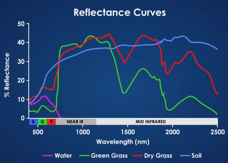
For example, vegetation has a distinct spectral signature.

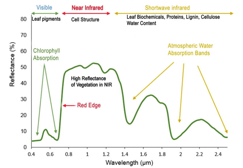
Vegetation has a unique spectral signature characterized by high reflectance in the near infrared wavelengths, and much lower reflectance in the green portion of the visible spectrum. For more details, refer to Vegetation Analysis: Using Vegetation Indices in ENVI. We can extract reflectance values in the NIR and visible spectrums from hyperspectral data in order to map vegetation on the earth's surface. You can also use spectral curves as a proxy for vegetation health. We will explore this concept more in the next lesson, where we will calculate vegetation indices.

Let's get started. First import the required packages.

import os
import dotenv
import neonutilities as nu
import numpy as np
import pandas as pd
import matplotlib.pyplot as plt
import requests
import sys

This next function provides a handy way to download the Python module that we will use in this lesson. This uses the requests package.

# function to download data stored on the internet in a public url to a local file
def download_url(url,download_dir):
    if not os.path.isdir(download_dir):
        os.makedirs(download_dir)
    filename = url.split('/')[-1]
    r = requests.get(url, allow_redirects=True)
    file_object = open(os.path.join(download_dir,filename),'wb')
    file_object.write(r.content)

Download the module from its location on GitHub, add the python_modules to the path and import the neon_aop_hyperspectral.py module.

module_url = "https://raw.githubusercontent.com/NEONScience/NEON-Data-Skills/main/tutorials/Python/AOP/aop_python_modules/neon_aop_hyperspectral.py"
download_url(module_url,'../python_modules')
# os.listdir('../python_modules') #optionally show the contents of this directory to confirm the file downloaded

sys.path.insert(0, '../python_modules')

# import the neon_aop_hyperspectral module
import neon_aop_hyperspectral as neon_hs;

Now that we've imported the required packages and the hyperspectral module, we can download a reflectance dataset using neonutilities and start to explore it. We'll download data from the NEON site Smithsonian Environmental Research Center (SERC). First, use nu.list_available_dates to find what years of data are available for the bidirectional reflectance dataset at SERC.

nu.list_available_dates('DP3.30006.002','SERC')

PROVISIONAL Available Dates: 2022-05, 2025-06

Here we can see the available dates for this dataset. Let's use data from 2025.

As of June 2026, NEON requires an API token for data downloads, to reduce bot scraping and improve user support. Tokens can be generated in NEON data portal user accounts - log in to your account or create one, and go to the API Tokens section. For best practices in storing and using tokens, follow the instructions here. Once you've set up your token as an environment variable, you can load it using the dotenv package as follows, optionally specifying the path to the .env file.

dotenv.load_dotenv()
token = os.environ.get("NEON_TOKEN")

Before downloading, we can check the extents in UTM x,y coordinates for the site as follows:

serc_2025_refl_exts = nu.get_aop_tile_extents('DP3.30006.002','SERC',2025,token=token)

Easting Bounds: (358000, 370000)
Northing Bounds: (4298000, 4312000)

For this example, download the reflectance tile with southwest coordinates of 368000, 4306000 using nu.by_tile_aop. Click y to continue the download after verifying the size (around 660 MB).

nu.by_tile_aop('DP3.30006.002',
               'SERC',
               2025,
               easting=368000,
               northing=4306000,
               token=token,
               include_provisional=True,
               savepath='C:/Data')

Provisional NEON data are included. To exclude provisional data, use input parameter include_provisional=False.


Continuing will download 2 NEON data files totaling approximately 661.3 MB. Do you want to proceed? (y/n)  y

The reflectance data tile is now downloaded into the 'C:/NEON_Data/DP3.30006.002' directory. You can use the code cell below to walk through all the directories and display where the .h5 file was downloaded.

# display .h5 data in the savepath
for root, dirs, files in os.walk(r'C:\Data\DP3.30006.002'):
    for file in files:
        if file.endswith(".h5"):
             h5_tile = os.path.join(root, file)
             print(h5_tile)

C:\Data\DP3.30006.002\neon-aop-provisional-products\2025\FullSite\D02\2025_SERC_7\L3\Spectrometer\Reflectance\NEON_D02_SERC_DP3_368000_4306000_bidirectional_reflectance.h5

# read in the data using the neon_hs module
serc_refl, serc_refl_md, wavelengths = neon_hs.aop_h5refl2array(h5_tile,'Reflectance')

Reading in  C:\Data\DP3.30006.002\neon-aop-provisional-products\2025\FullSite\D02\2025_SERC_7\L3\Spectrometer\Reflectance\NEON_D02_SERC_DP3_368000_4306000_bidirectional_reflectance.h5

Optionally, you can view the data stored in the metadata dictionary, and print the minimum, maximum, and mean reflectance values in the tile. In order to ignore NaN values, use numpy.nanmin/nanmax/nanmean.

for item in sorted(serc_refl_md):
    print(item + ':',serc_refl_md[item])

print('\nSERC Tile Reflectance Stats:')
print('min:',np.nanmin(serc_refl))
print('max:',round(np.nanmax(serc_refl),2))
print('mean:',round(np.nanmean(serc_refl),2))

EPSG: 32618
bad_band_window1: [1340 1445]
bad_band_window2: [1790 1955]
ext_dict: {'xMin': 368000.0, 'xMax': 369000.0, 'yMin': 4306000.0, 'yMax': 4307000.0}
extent: (368000.0, 369000.0, 4306000.0, 4307000.0)
no_data_value: -9999.0
projection: b'+proj=UTM +zone=18 +ellps=WGS84 +datum=WGS84 +units=m +no_defs'
res: {'pixelWidth': 1.0, 'pixelHeight': 1.0}
scale_factor: 10000.0
shape: (1000, 1000, 426)
source: C:\Data\DP3.30006.002\neon-aop-provisional-products\2025\FullSite\D02\2025_SERC_7\L3\Spectrometer\Reflectance\NEON_D02_SERC_DP3_368000_4306000_bidirectional_reflectance.h5

SERC Tile Reflectance Stats:
min: -100
max: 15599
mean: 1219.84

For reference, plot the red band of the tile, using splicing, and the plot_aop_refl function:

sercb56 = serc_refl[:,:,55]/serc_refl_md['scale_factor']

neon_hs.plot_aop_refl(sercb56,
                      serc_refl_md['extent'],
                      colorlimit=(0,0.3),
                      title='SERC Tile Band 56',
                      cmap_title='Reflectance',
                      colormap='gist_earth')

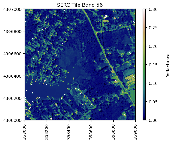
We can use pandas to create a dataframe containing the wavelength and reflectance values for a single pixel - in this example, we'll look at the center pixel of the tile (500,500). To extract all reflectance values from a single pixel, use splicing as we did before to select a single band, but now we need to specify (y,x) and select all bands (using :).

serc_pixel_df = pd.DataFrame()
serc_pixel_df['reflectance'] = serc_refl[500,500,:]/serc_refl_md['scale_factor']
serc_pixel_df['wavelengths'] = wavelengths

We can preview the first and last five values of the dataframe using head and tail:

print(serc_pixel_df.head(5))
print(serc_pixel_df.tail(5))

   reflectance  wavelengths
0       0.0126   381.858398
1       0.0255   386.868896
2       0.0260   391.879395
3       0.0232   396.889893
4       0.0216   401.900391
     reflectance  wavelengths
421       0.5233  2491.281494
422       0.2784  2496.291992
423       0.1952  2501.302490
424       0.7879  2506.312988
425       1.4948  2511.323486

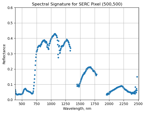
We can now plot the spectra, stored in this dataframe structure. pandas has a built in plotting routine, which can be called by typing .plot at the end of the dataframe.

serc_pixel_df.plot(x='wavelengths',y='reflectance',kind='scatter',edgecolor='none')
plt.title('Spectral Signature for SERC Pixel (500,500)')
ax = plt.gca() 
ax.set_xlim([np.min(serc_pixel_df['wavelengths']),np.max(serc_pixel_df['wavelengths'])])
ax.set_ylim(0,0.6)
ax.set_xlabel("Wavelength, nm")
ax.set_ylabel("Reflectance")
ax.grid('on')

Water Vapor Band Windows

We can see from the spectral profile above that there are spikes in reflectance around ~1400nm and ~1800nm. These result from water vapor which absorbs light between wavelengths 1340-1445 nm and 1790-1955 nm. The atmospheric correction that converts radiance to reflectance subsequently results in a spike at these two bands. The wavelengths of these water vapor bands is stored in the reflectance attributes, which is saved in the reflectance metadata dictionary created with h5refl2array:

bbw1 = serc_refl_md['bad_band_window1']; 
bbw2 = serc_refl_md['bad_band_window2']; 
print('Bad Band Window 1:',bbw1)
print('Bad Band Window 2:',bbw2)

Bad Band Window 1: [1340 1445]
Bad Band Window 2: [1790 1955]

Below we repeat the plot we made above, but this time draw in the edges of the water vapor band windows that we need to remove.

serc_pixel_df.plot(x='wavelengths',y='reflectance',kind='scatter',edgecolor='none');
plt.title('Spectral Signature for SERC Pixel (500,500)')
ax1 = plt.gca(); ax1.grid('on')
ax1.set_xlim([np.min(serc_pixel_df['wavelengths']),np.max(serc_pixel_df['wavelengths'])]); 
ax1.set_ylim(0,0.5)
ax1.set_xlabel("Wavelength, nm"); ax1.set_ylabel("Reflectance")

#Add in red dotted lines to show boundaries of bad band windows:
ax1.plot((1340,1340),(0,1.5), 'r--');
ax1.plot((1445,1445),(0,1.5), 'r--');
ax1.plot((1790,1790),(0,1.5), 'r--');
ax1.plot((1955,1955),(0,1.5), 'r--');

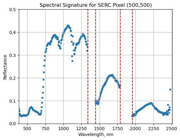
We can now set these bad band windows to nan, along with the last 10 bands, which are also often noisy (as seen in the spectral profile plotted above). First make a copy of the wavelengths so that the original metadata doesn't change.

w = wavelengths.copy() #make a copy to deal with the mutable data type
w[((w >= 1340) & (w <= 1445)) | ((w >= 1790) & (w <= 1955))]=np.nan #can also use bbw1[0] or bbw1[1] to avoid hard-coding in
w[-10:]=np.nan;  # the last 10 bands sometimes have noise - best to eliminate
#print(w) #optionally print wavelength values to show that -9999 values are replaced with nan

Interactive Spectra Visualization

Finally, we can create a widget to interactively view the spectra of different pixels along the reflectance tile. Run the cell below, and select different pixel_x and pixel_y values to gain a sense of what the spectra look like for different materials on the ground.

from ipywidgets import interact

# --- Data Initialization Setup ---
# define refl_band, refl, and metadata, as copies of the original serc_refl data
refl_band = sercb56
refl = serc_refl.copy()
metadata = serc_refl_md.copy()

# pre-extract coordinate mapping info
ext = metadata['extent']

def interactive_spectra_plot(pixel_x, pixel_y):
    # extract reflectance vector for the targeted pixel
    reflectance = refl[pixel_y, pixel_x, :]
    
    # make pixel dataframe
    pixel_df = pd.DataFrame({
        'reflectance': reflectance,
        'wavelengths': w
    })

    # figure set-up
    fig, (ax1, ax2) = plt.subplots(1, 2, figsize=(15, 5))

    # --- Plot 1: Spectra Scatter ---
    pixel_df.plot(
        ax=ax1, 
        x='wavelengths', 
        y='reflectance', 
        kind='scatter', 
        edgecolor='none'
    )
    
    ax1.set_title(f"Spectra of Pixel ({pixel_x}, {pixel_y})")
    ax1.set_xlabel("Wavelength, nm")
    ax1.set_ylabel("Reflectance")
    ax1.set_xlim([np.min(wavelengths), np.max(wavelengths)])
    ax1.set_ylim([np.min(reflectance), np.max(reflectance) * 1.1])
    ax1.grid(True)  # FIX: Changed from 'on' to True for modern Python/Matplotlib

    # --- Plot 2: Pixel Location Map ---
    plot = ax2.imshow(refl_band, extent=ext, cmap='gist_earth', clim=(0, 0.1))
    ax2.set_title('Pixel Location')
    
    # colorbar
    cbar = fig.colorbar(plot, ax=ax2, aspect=20)
    cbar.set_label('Reflectance', rotation=90, labelpad=20)
    
    # tick adjustments
    ax2.ticklabel_format(useOffset=False, style='plain')
    ax2.tick_params(axis='x', labelrotation=90) # FIX: Avoided old plt.setp logic
    
    # calculate coordinate markers
    marker_x = ext[0] + pixel_x
    marker_y = ext[3] - pixel_y
    ax2.plot(marker_x, marker_y, marker='s', markersize=5, color='red')
    
    ax2.set_xlim(ext[0], ext[1])
    ax2.set_ylim(ext[2], ext[3])
    
    plt.show() 

# --- Run Interactive UI ---
interact(
    interactive_spectra_plot, 
    pixel_x=(0, refl.shape[1] - 1, 1),
    pixel_y=(0, refl.shape[0] - 1, 1)
);