Tutorial
Plot Spectral Signatures Derived from Hyperspectral Remote Sensing Data in HDF5 Format in R
Last Updated: Apr 2, 2026
Learning Objectives
After completing this tutorial, you will be able to:
- Extract and plot a single spectral signature from an HDF5 file.
- Work with groups and datasets within an HDF5 file.
Things You’ll Need To Complete This Tutorial
To complete this tutorial you will need the most current version of R and, preferably, RStudio loaded on your computer.
R Libraries to Install:
-
rhdf5:
install.packages("BiocManager"),BiocManager::install("rhdf5") -
plyr:
install.packages('plyr') -
ggplot2:
install.packages('ggplot2') -
neonUtilities:
install.packages('neonUtilities')
More on Packages in R - Adapted from Software Carpentry.
Data
These hyperspectral remote sensing data provide information on the National Ecological Observatory Network's San Joaquin Experimental Range (SJER) field site in March of 2021. The data used in this lesson is the 1km by 1km mosaic tile named NEON_D17_SJER_DP3_257000_4112000_reflectance.h5. If you already completed the previous lesson in this tutorial series, you do not need to download this data again. The entire SJER reflectance dataset can be accessed from the NEON Data Portal.
Set Working Directory: This lesson assumes that you have set your working directory to the location of the downloaded and unzipped data subsets.
An overview of setting the working directory in R can be found here.
Recommended Skills
For this tutorial, you should be comfortable reading data from a HDF5 file and have a general familiarity with hyperspectral data. If you aren't familiar with these steps already, we highly recommend you work through the Introduction to Working with Hyperspectral Data in HDF5 Format in R tutorial before moving on to this tutorial.
Everything on our planet reflects electromagnetic radiation from the Sun, and different types of land cover often have dramatically different reflectance properties across the spectrum. One of the most powerful aspects of the NEON Imaging Spectrometer (NIS, or hyperspectral sensor) is that it can accurately measure these reflectance properties at a very high spectral resolution. When you plot the reflectance values across the observed spectrum, you will see that different land cover types (vegetation, pavement, bare soils, etc.) have distinct patterns in their reflectance values, a property that we call the 'spectral signature' of a particular land cover class.
In this tutorial, we will extract the reflectance values for all bands of a single pixel to plot a spectral signature for that pixel. In order to do this, we need to pair the reflectance values for that pixel with the wavelength values of the bands that are represented in those measurements. We will also need to adjust the reflectance values by the scaling factor that is saved as an 'attribute' in the HDF5 file. First, let's start by defining the working directory and reading in the example dataset.
# Call required packages

library(rhdf5)

library(plyr)

library(ggplot2)

library(neonUtilities)


wd <- "~/data/" #This will depend on your local environment

setwd(wd)
If you haven't already downloaded the hyperspectral data tile (in one of the previous tutorials in this series), you can use the neonUtilities function byTileAOP to download a single reflectance tile. You can run help(byTileAOP) to see more details on what the various inputs are. For this exercise, we'll specify the UTM Easting and Northing to be (257500, 4112500), which will download the tile with the lower left corner (257000, 4112000).
byTileAOP(dpID = 'DP3.30006.001',

          site = 'SJER',

          year = '2021',

          easting = 257500,

          northing = 4112500,

          savepath = wd)
This file will be downloaded into a nested subdirectory under the ~/data folder (your working directory), inside a folder named DP3.30006.001 (the Data Product ID). The file should show up in this location: ~/data/DP3.30006.001/neon-aop-products/2021/FullSite/D17/2021_SJER_5/L3/Spectrometer/Reflectance/NEON_D17_SJER_DP3_257000_4112000_reflectance.h5.
Now we can read in the file and look at the contents using h5ls. You can move this file to a different location, but make sure to change the path accordingly.
# define the h5 file name (specify the full path)

h5_file <- paste0(wd,"DP3.30006.001/neon-aop-products/2021/FullSite/D17/2021_SJER_5/L3/Spectrometer/Reflectance/NEON_D17_SJER_DP3_257000_4112000_reflectance.h5")


# look at the HDF5 file structure

h5ls(h5_file) #optionally specify all=True if you want to see all of the information

##                                           group                                 name       otype  dclass               dim
## 0                                             /                                 SJER   H5I_GROUP
## 1                                         /SJER                          Reflectance   H5I_GROUP
## 2                             /SJER/Reflectance                             Metadata   H5I_GROUP
## 3                    /SJER/Reflectance/Metadata                    Ancillary_Imagery   H5I_GROUP
## 4  /SJER/Reflectance/Metadata/Ancillary_Imagery                Aerosol_Optical_Depth H5I_DATASET INTEGER       1000 x 1000
## 5  /SJER/Reflectance/Metadata/Ancillary_Imagery                               Aspect H5I_DATASET   FLOAT       1000 x 1000
## 6  /SJER/Reflectance/Metadata/Ancillary_Imagery                          Cast_Shadow H5I_DATASET INTEGER       1000 x 1000
## 7  /SJER/Reflectance/Metadata/Ancillary_Imagery Dark_Dense_Vegetation_Classification H5I_DATASET INTEGER       1000 x 1000
## 8  /SJER/Reflectance/Metadata/Ancillary_Imagery                 Data_Selection_Index H5I_DATASET INTEGER       1000 x 1000
## 9  /SJER/Reflectance/Metadata/Ancillary_Imagery                 Haze_Cloud_Water_Map H5I_DATASET INTEGER       1000 x 1000
## 10 /SJER/Reflectance/Metadata/Ancillary_Imagery                  Illumination_Factor H5I_DATASET INTEGER       1000 x 1000
## 11 /SJER/Reflectance/Metadata/Ancillary_Imagery                          Path_Length H5I_DATASET   FLOAT       1000 x 1000
## 12 /SJER/Reflectance/Metadata/Ancillary_Imagery                      Sky_View_Factor H5I_DATASET INTEGER       1000 x 1000
## 13 /SJER/Reflectance/Metadata/Ancillary_Imagery                                Slope H5I_DATASET   FLOAT       1000 x 1000
## 14 /SJER/Reflectance/Metadata/Ancillary_Imagery             Smooth_Surface_Elevation H5I_DATASET   FLOAT       1000 x 1000
## 15 /SJER/Reflectance/Metadata/Ancillary_Imagery                 Visibility_Index_Map H5I_DATASET INTEGER       1000 x 1000
## 16 /SJER/Reflectance/Metadata/Ancillary_Imagery                   Water_Vapor_Column H5I_DATASET   FLOAT       1000 x 1000
## 17 /SJER/Reflectance/Metadata/Ancillary_Imagery            Weather_Quality_Indicator H5I_DATASET INTEGER   3 x 1000 x 1000
## 18                   /SJER/Reflectance/Metadata                    Coordinate_System   H5I_GROUP
## 19 /SJER/Reflectance/Metadata/Coordinate_System             Coordinate_System_String H5I_DATASET  STRING             ( 0 )
## 20 /SJER/Reflectance/Metadata/Coordinate_System                            EPSG Code H5I_DATASET  STRING             ( 0 )
## 21 /SJER/Reflectance/Metadata/Coordinate_System                             Map_Info H5I_DATASET  STRING             ( 0 )
## 22 /SJER/Reflectance/Metadata/Coordinate_System                                Proj4 H5I_DATASET  STRING             ( 0 )
## 23                   /SJER/Reflectance/Metadata                    Flight_Trajectory   H5I_GROUP
## 24                   /SJER/Reflectance/Metadata                                 Logs   H5I_GROUP
## 25              /SJER/Reflectance/Metadata/Logs                               195724   H5I_GROUP
## 26       /SJER/Reflectance/Metadata/Logs/195724                     ATCOR_Input_file H5I_DATASET  STRING             ( 0 )
## 27       /SJER/Reflectance/Metadata/Logs/195724                 ATCOR_Processing_Log H5I_DATASET  STRING             ( 0 )
## 28       /SJER/Reflectance/Metadata/Logs/195724                Shadow_Processing_Log H5I_DATASET  STRING             ( 0 )
## 29       /SJER/Reflectance/Metadata/Logs/195724               Skyview_Processing_Log H5I_DATASET  STRING             ( 0 )
## 30       /SJER/Reflectance/Metadata/Logs/195724                  Solar_Azimuth_Angle H5I_DATASET   FLOAT             ( 0 )
## 31       /SJER/Reflectance/Metadata/Logs/195724                   Solar_Zenith_Angle H5I_DATASET   FLOAT             ( 0 )
## 32              /SJER/Reflectance/Metadata/Logs                               200251   H5I_GROUP
## 33       /SJER/Reflectance/Metadata/Logs/200251                     ATCOR_Input_file H5I_DATASET  STRING             ( 0 )
## 34       /SJER/Reflectance/Metadata/Logs/200251                 ATCOR_Processing_Log H5I_DATASET  STRING             ( 0 )
## 35       /SJER/Reflectance/Metadata/Logs/200251                Shadow_Processing_Log H5I_DATASET  STRING             ( 0 )
## 36       /SJER/Reflectance/Metadata/Logs/200251               Skyview_Processing_Log H5I_DATASET  STRING             ( 0 )
## 37       /SJER/Reflectance/Metadata/Logs/200251                  Solar_Azimuth_Angle H5I_DATASET   FLOAT             ( 0 )
## 38       /SJER/Reflectance/Metadata/Logs/200251                   Solar_Zenith_Angle H5I_DATASET   FLOAT             ( 0 )
## 39              /SJER/Reflectance/Metadata/Logs                               200812   H5I_GROUP
## 40       /SJER/Reflectance/Metadata/Logs/200812                     ATCOR_Input_file H5I_DATASET  STRING             ( 0 )
## 41       /SJER/Reflectance/Metadata/Logs/200812                 ATCOR_Processing_Log H5I_DATASET  STRING             ( 0 )
## 42       /SJER/Reflectance/Metadata/Logs/200812                Shadow_Processing_Log H5I_DATASET  STRING             ( 0 )
## 43       /SJER/Reflectance/Metadata/Logs/200812               Skyview_Processing_Log H5I_DATASET  STRING             ( 0 )
## 44       /SJER/Reflectance/Metadata/Logs/200812                  Solar_Azimuth_Angle H5I_DATASET   FLOAT             ( 0 )
## 45       /SJER/Reflectance/Metadata/Logs/200812                   Solar_Zenith_Angle H5I_DATASET   FLOAT             ( 0 )
## 46              /SJER/Reflectance/Metadata/Logs                               201441   H5I_GROUP
## 47       /SJER/Reflectance/Metadata/Logs/201441                     ATCOR_Input_file H5I_DATASET  STRING             ( 0 )
## 48       /SJER/Reflectance/Metadata/Logs/201441                 ATCOR_Processing_Log H5I_DATASET  STRING             ( 0 )
## 49       /SJER/Reflectance/Metadata/Logs/201441                Shadow_Processing_Log H5I_DATASET  STRING             ( 0 )
## 50       /SJER/Reflectance/Metadata/Logs/201441               Skyview_Processing_Log H5I_DATASET  STRING             ( 0 )
## 51       /SJER/Reflectance/Metadata/Logs/201441                  Solar_Azimuth_Angle H5I_DATASET   FLOAT             ( 0 )
## 52       /SJER/Reflectance/Metadata/Logs/201441                   Solar_Zenith_Angle H5I_DATASET   FLOAT             ( 0 )
## 53                   /SJER/Reflectance/Metadata                        Spectral_Data   H5I_GROUP
## 54     /SJER/Reflectance/Metadata/Spectral_Data                                 FWHM H5I_DATASET   FLOAT               426
## 55     /SJER/Reflectance/Metadata/Spectral_Data                           Wavelength H5I_DATASET   FLOAT               426
## 56                   /SJER/Reflectance/Metadata              to-sensor_azimuth_angle H5I_DATASET   FLOAT       1000 x 1000
## 57                   /SJER/Reflectance/Metadata               to-sensor_zenith_angle H5I_DATASET   FLOAT       1000 x 1000
## 58                            /SJER/Reflectance                     Reflectance_Data H5I_DATASET INTEGER 426 x 1000 x 1000
Read Wavelength Values
Next, let's read in the wavelength center associated with each band in the HDF5 file. We will later match these with the reflectance values and show both in our final spectral signature plot.
# read in the wavelength information from the HDF5 file

wavelengths <- h5read(h5_file,"/SJER/Reflectance/Metadata/Spectral_Data/Wavelength")
Extract Z-dimension data slice
Next, we will extract all reflectance values for one pixel. This makes up the spectral signature or profile of the pixel. To do that, we'll use the h5read() function. Here we pick an arbitrary pixel at (100,35), and use the NULL value to select all bands from that location.
# extract all bands from a single pixel

aPixel <- h5read(h5_file,"/SJER/Reflectance/Reflectance_Data",index=list(NULL,100,35))


# The line above generates a vector of reflectance values.

# Next, we reshape the data and turn them into a dataframe

b <- adply(aPixel,c(1))


# create clean data frame

aPixeldf <- b[2]


# add wavelength data to matrix

aPixeldf$Wavelength <- wavelengths


head(aPixeldf)

##    V1 Wavelength
## 1 206   381.6035
## 2 266   386.6132
## 3 274   391.6229
## 4 297   396.6327
## 5 236   401.6424
## 6 236   406.6522
Scale Factor
Then, we can pull the spatial attributes that we'll need to adjust the reflectance values. Often, large raster data contain floating point (values with decimals) information. However, floating point data consume more space (yield a larger file size) compared to integer values. Thus, to keep the file sizes smaller, the data will be scaled by a factor of 10, 100, 10000, etc. This scale factor will be noted in the data attributes.
# grab scale factor from the Reflectance attributes

reflectanceAttr <- h5readAttributes(h5_file,"/SJER/Reflectance/Reflectance_Data" )


scaleFact <- reflectanceAttr$Scale_Factor


# add scaled data column to DF

aPixeldf$scaled <- (aPixeldf$V1/as.vector(scaleFact))


# make nice column names

names(aPixeldf) <- c('Reflectance','Wavelength','ScaledReflectance')

head(aPixeldf)

##   Reflectance Wavelength ScaledReflectance
## 1         206   381.6035            0.0206
## 2         266   386.6132            0.0266
## 3         274   391.6229            0.0274
## 4         297   396.6327            0.0297
## 5         236   401.6424            0.0236
## 6         236   406.6522            0.0236
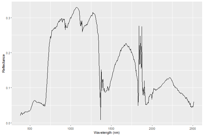
Plot Spectral Signature
Now we're ready to plot our spectral signature!
ggplot(data=aPixeldf)+
   geom_line(aes(x=Wavelength, y=ScaledReflectance))+
   xlab("Wavelength (nm)")+
   ylab("Reflectance")