NEON Domain and Site Shapefiles and Maps

This tutorial explores NEON domain- and site-level spatial data, using shapefiles and tabular data provided by the NEON project. The intent of this tutorial is to provide guidance in navigating the data and files provided by NEON, and in creating maps of the domain and site locations. We hope these data and methods will assist users in generating images and figures for publications or presentations related to NEON.

Setup R Environment

We'll use the sf R package in this tutorial. Install the package, if not already installed, and load the library.

# run once to get the package, and re-run if you need to get updates

install.packages("sf")  # work with spatial data



# run every time you start a script

library(sf)



# set working directory to ensure R can find the file we wish to import and where

# we want to save our files. 



wd <- "~/data/" # This will depend on your local environment

setwd(wd)

NEON spatial data files

NEON spatial data are available in a number of different files depending on which spatial data you are interested in. This section covers a variety of spatial data files that can be directly downloaded from the NEONScience.org website instead of being delivered with a downloaded data product.

The goal of this section is to create a map of the entire Observatory that includes the NEON domain boundaries and differentiates between aquatic and terrestrial field sites.

Site locations & domain boundaries

Most NEON spatial data files that are not part of the data downloads are available on the Spatial Data and Maps page as both shapefiles and kmz files.

In addition, latitude, longitude, elevation, and some other basic metadata for each site are available for download from the Field Sites page on the NEON website (linked above the image). In this summary of each field site, the geographic coordinates for each site correspond to the tower location for terrestrial sites and the center of the permitted reach for aquatic sites.

To continue, please download these files from the NEON website:

• NEON Domain Polygons: A polygon shapefile defining NEON's domain boundaries. Like all NEON data the Coordinate Reference system is Geographic WGS 84. Available on the Spatial Data and Maps page.
• Field Site csv: generic locations data for each NEON field site. Available on the Field Sites page.

The Field Site location data is also available as a shapefile and KMZ on the Spatial Data and Maps page. We use the file from the site list to demonstrate alternative ways to work with spatial data.

Map NEON domains

Using the domain shapefile and the field sites list, let's make a map of NEON site locations.

We'll read in the spatial data using the sf package and plot it using base R. First, read in the domain shapefile.

Be sure to move the downloaded and unzipped data files into the working directory you set earlier!

# upload data

neonDomains <- read_sf(paste0(wd,"NEONDomains_2024"), layer="NEON_Domains")

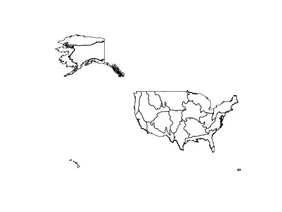
The data come as a Large SpatialPolygonsDataFrame. Base R has methods for working with this data type, and will recognize it automatically with the generic plot() function. Let's first plot the domains without the sites.

plot(st_geometry(neonDomains))

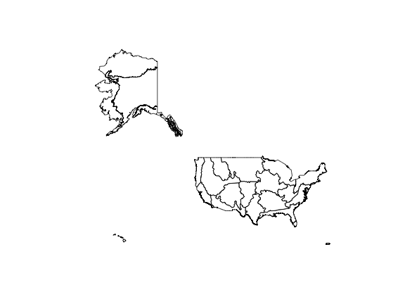
The data are currently in a Lat-Long projection. The map will look a little more familiar if we convert it to a Mercator projection. There are many, many map projections possible, and Mercator is distorted in very well-documented ways! Here, we'll use it as a demonstration, but you may want to use a different projection in your own work.

The st_transform() function in the sf package can be used to convert the projection:

neonMercator <- st_transform(neonDomains,
                            crs="+proj=merc")

plot(st_geometry(neonMercator))

Map NEON field sites

Now that we have a map of all the NEON domains, let's plot the NEON field site locations on it. To do this, we need to load and explore the field sites data.

# read in the data

# make sure the file name matches the file you downloaded

# the date stamp is updated over time

neonSites <- read.delim(paste0(wd,"NEON_Field_Site_Metadata_20241219.csv"), 
                        sep=",", header=T)



# view data structure for each variable

str(neonSites)

## 'data.frame':	81 obs. of  42 variables:
##  $ field_domain_id                   : chr  "D16" "D10" "D03" "D18" ...
##  $ field_site_id                     : chr  "ABBY" "ARIK" "BARC" "BARR" ...
##  $ field_site_name                   : chr  "Abby Road NEON" "Arikaree River NEON" "Lake Barco NEON" "Utqiaġvik NEON" ...
##  $ field_site_type                   : chr  "Gradient Terrestrial" "Core Aquatic" "Core Aquatic" "Gradient Terrestrial" ...
##  $ field_site_subtype                : chr  "" "Wadeable Stream" "Lake" "" ...
##  $ field_colocated_site              : chr  "" "" "OSBS" "" ...
##  $ field_site_host                   : chr  "Washington Department of Natural Resources" "The Nature Conservancy|Fox Ranch" "University of Florida Foundation" "Ukpeagvik Inupiat Corporation" ...
##  $ field_site_url                    : chr  "https://www.dnr.wa.gov/" "https://www.nature.org/en-us/get-involved/how-to-help/places-we-protect/fox-ranch/|https://www.nature.org/en-us"| __truncated__ "https://ordway-swisher.ufl.edu/ResearchUse.aspx" "http://www.north-slope.org/departments/planning-community-services/applications-and-forms" ...
##  $ field_nonneon_research_allowed    : chr  "No" "Yes" "Yes" "Yes" ...
##  $ field_latitude                    : num  45.8 39.8 29.7 71.3 44.1 ...
##  $ field_longitude                   : num  -122.3 -102.4 -82 -156.6 -71.3 ...
##  $ field_geodetic_datum              : chr  "WGS84" "WGS84" "WGS84" "WGS84" ...
##  $ field_utm_northing                : num  5067870 4404043 3283363 7910572 4881512 ...
##  $ field_utm_easting                 : num  552076 718694 402359 585246 316812 ...
##  $ field_utm_zone                    : chr  "10N" "13N" "17N" "4N" ...
##  $ field_site_county                 : chr  "Clark" "Yuma" "Putnam" "North Slope" ...
##  $ field_site_state                  : chr  "WA" "CO" "FL" "AK" ...
##  $ field_site_country                : chr  "US" "US" "US" "US" ...
##  $ field_mean_evelation_m            : int  365 1179 27 4 274 1197 183 2053 289 22 ...
##  $ field_minimum_elevation_m         : int  NA NA NA 0 230 NA 119 NA NA NA ...
##  $ field_maximum_elevation_m         : int  708 NA NA 13 655 NA 193 NA NA NA ...
##  $ field_mean_annual_temperature_C   : chr  "10.0°C" "10.4°C" "20.9°C" "-12.0°C" ...
##  $ field_mean_annual_precipitation_mm: int  2451 452 1308 105 1325 900 983 481 1041 1372 ...
##  $ field_dominant_wind_direction     : chr  "" "" "" "E" ...
##  $ field_mean_canopy_height_m        : num  34 NA NA 0.3 23 NA 1 NA NA NA ...
##  $ field_dominant_nlcd_classes       : chr  "Evergreen Forest|Grassland/Herbaceous|Shrub/Scrub" "Emergent Herbaceous Wetlands|Grassland/Herbaceous|Woody Wetlands" "Shrub/Scrub" "Emergent Herbaceous Wetlands" ...
##  $ field_dominant_plant_species      : logi  NA NA NA NA NA NA ...
##  $ field_usgs_huc                    : chr  "" "[h10250001](https://water.usgs.gov/lookup/getwatershed?10250001)" "[h03080103](https://water.usgs.gov/lookup/getwatershed?03080103)" "" ...
##  $ field_watership_name              : chr  "" "Lower Sappa" "Lower St. Johns" "" ...
##  $ field_watership_size_km2          : num  NA 2631.8 31.3 NA NA ...
##  $ field_lake_depth_mean_m           : num  NA NA 3.3 NA NA NA NA NA NA NA ...
##  $ field_lake_depth_max_m            : num  NA NA 6.7 NA NA NA NA NA NA NA ...
##  $ field_tower_height_m              : int  19 NA NA 9 35 NA 8 NA NA NA ...
##  $ field_megapit_soil_family         : chr  "Fine-lomay - isotic - mesic - Andic Humudepts" "" "" "Fine-silty - mixed - superactive - nonacid - pergelic Typic Histoturbels" ...
##  $ field_soil_subgroup               : chr  "Andic Humudepts" "" "" "Typic Histoturbels" ...
##  $ field_avg_number_of_green_days    : int  190 NA NA 45 180 NA 235 NA NA NA ...
##  $ field_avg_green_increase_doy      : int  110 NA NA 175 120 NA 75 NA NA NA ...
##  $ field_avg_green_max_doy           : int  165 NA NA 195 170 NA 150 NA NA NA ...
##  $ field_avg_green_decrease_doy      : int  205 NA NA 210 220 NA 210 NA NA NA ...
##  $ field_avg_green_min_doy           : chr  "300" "" "" "220" ...
##  $ field_phenocams                   : chr  "One phenocam is attached to the top and the bottom of the tower.\nhttps://phenocam.nau.edu/webcam/sites/NEON.D1"| __truncated__ "A phenocam is pointed toward the land-water interface of the site.\nhttps://phenocam.nau.edu/webcam/sites/NEON."| __truncated__ "A phenocam is pointed toward the land-water interface of the site.\nhttps://phenocam.nau.edu/webcam/sites/NEON."| __truncated__ "One phenocam is attached to the top and the bottom of the tower.\nhttps://phenocam.nau.edu/webcam/sites/NEON.D1"| __truncated__ ...
##  $ field_number_tower_levels         : int  5 NA NA 4 6 NA 4 NA NA NA ...

Here there is a lot of associated data about the field sites that may be of interest, such as site descriptions and dominant vegetation types. For mapping purposes, we can see that there are both latitude and longitude data, so we can plot this data onto our previous map.

plot(st_geometry(neonDomains))

points(neonSites$field_latitude~neonSites$field_longitude,
       pch=20)

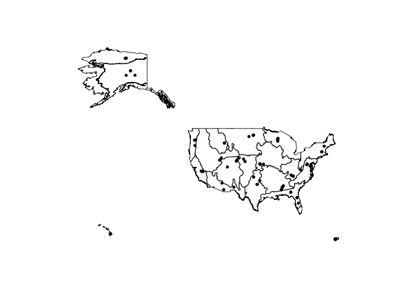
Now we can see all the sites across the Observatory. Note that we've switched back to the Lat-Long projection, which makes it simple to plot the site locations onto the map using their latitude and longitude. To plot them on the Mercator projection, we would need to perform the same conversion on the coordinates. See sf package documentation if you are interested in doing this.

NEON has both aquatic and terrestrial sites, with important differences between the two. Looking back at the variables in this data set, we can see that field_site_type designates the aquatic and terrestrial sites.

Let's differentiate the site types by adding color to our plot, with terrestrial sites in green and aquatic sites in blue.

# create empty variable

siteCol <- character(nrow(neonSites))



# populate new variable with colors, according to Site.Type

siteCol[grep("Aquatic", neonSites$field_site_type)] <- "blue"

siteCol[grep("Terrestrial", neonSites$field_site_type)] <- "green"



# add color to points on map

plot(st_geometry(neonDomains))

points(neonSites$field_latitude~neonSites$field_longitude,
       pch=20, col=siteCol)

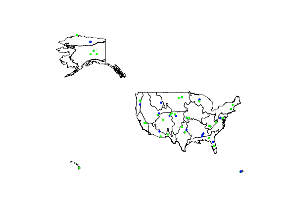
Now we can see where NEON sites are located within the domains. Note that a significant number of terrestrial and aquatic sites are co-located; in those cases both sites are plotted here, but one color may be superimposed over the other.

Map locations at a specific site

Also available on the Spatial Data and Maps page are shapefiles containing location data at the within-site level.

If you are interested in maps of NEON sampling locations and regions, explore the downloads available for Terrestrial Observation Sampling Locations, Flight Boundaries, and Aquatic Sites Watersheds. These downloads contain shapefiles of these locations, and the terrestrial sampling file also contains spatial data in tabular form.

If you are interested in learning how to work with sampling location data that are provided along with downloads of NEON sensor and observational data, see the Geolocation Data tutorial.