
Tutorial
Estimating Bird Occupancy and Detection Using NEON Observational Data
Last Updated: Jul 8, 2026
This tutorial explores the use of NEON breeding landbird data for occupancy modeling. The focus is on building detection histories from observational data, fitting a simple occupancy model, and testing how site and survey conditions may influence occupancy and detection.
Although birds are used here, the same workflow could be applied to other observational sampling datasets that provide species-level detections, such as small mammals or fish. Environmental covariates for these models can also be drawn from other NEON data products, such as weather and climate measurements collected by NEON's Automated Instrument Systems.
Learning Objectives
After completing this tutorial you will be able to:
- Understand the basics of occupancy modeling.
- Build detection histories of NEON breeding landbird data.
- Fit occupancy models in R and interpret occupancy and detection estimates.
- Incorporate site-level and survey-level environmental covariates to evaluate factors influencing detection and occupancy.
Things You’ll Need To Complete This Tutorial
R Programming Language
You will need a current version of R to complete this tutorial. We also recommend the RStudio IDE to work with R.
Introduction to NEON Bird Observations
NEON’s breeding landbird point count dataset provides taxonomic identifications, detection methods, and associated survey and site information for birds observed during standardized six-minute surveys. The protocol focuses on diurnal, terrestrial breeding landbirds, a group chosen because they respond strongly to changes in climate, habitat, and land use.
Field crews survey spatially distributed plots across NEON field sites during the breeding season every year, recording every bird seen or heard. These repeated surveys produce rich detection–nondetection data suited for occupancy modeling.
NEON’s terrestrial field sites are designated as large or small, which determines the sampling design. Large sites are surveyed once per year and contain 5–10 plots each containing a bird grid, made up of a 3×3 array of nine points spaced 250 m apart (see Figure 1). Field crews visit every point in a grid and conduct a 6-minute point-count survey. Smaller sites, which cannot accommodate full grids, contain 2–25 point-count locations randomly distributed across the site and spaced at least 250 m apart. These are surveyed twice per year.
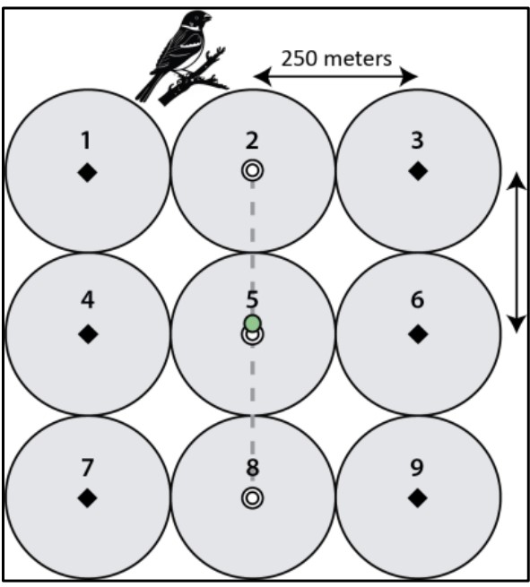
More details on NEON’s bird monitoring program are available on the NEON bird resource page. Protocols referenced in the data can be found in the Document Library.
Introduction to Occupancy Modeling
When searching for a species, there are technically three possible outcomes:
- The species is present and you detect it,
- the species is present and you do not detect it, or
- the species is absent and therefore not detected.
Traditional presence–absence data cannot distinguish missed detections from true absences. Occupancy modeling addresses this challenge by explicitly modeling two linked processes: the true occupancy of the species and the probability of detecting the species given that it is present. A key assumption of occupancy modeling is closure during the sampling period: the true occupancy state of a site does not change between repeated surveys.
This framework estimates two key parameters:
- the probability that a site is occupied by a species, i.e., occupancy (ψ)
- the probability of detecting the species during a survey, given that it is present, i.e., detection (p).
To tease apart ψ and p, occupancy models require repeated surveys of the same site. NEON’s observational sampling design is ideal for this approach, because surveys include repeated, standardized visits to locations across time.
Setup R Environment
We'll need several R packages in this tutorial. Install the packages, if not already installed, and load the libraries for each.
# run once to get the package, and re-run if you need to get updates

install.packages("neonUtilities") # work with NEON data

install.packages('RPresence', repo='https://www.mbr-pwrc.usgs.gov/mbrCRAN') # library for occupancy modelling

install.packages("dplyr") # data manipulation

install.packages("tidyr") # data reshaping and tidying

install.packages("stringr") # string handling and text processing

install.packages("ggplot2") # visualization and plotting


# load the libraries into your environment

library(neonUtilities)

library(RPresence)

library(dplyr)

library(tidyr)

library(stringr)

library(ggplot2)
Importing NEON Data
First, we’ll download the breeding landbird data product (DP1.10003.001) for all NEON terrestrial field sites included in RELEASE-2026.
- NEON (National Ecological Observatory Network). Breeding landbird point counts (DP1.10003.001), RELEASE-2026. https://doi.org/10.48443/v6hs-mx57. Dataset accessed in R via neonUtilities on .
On the first run, this code block will download the full dataset for all sites. Because the data product is large and spans multiple years-including years before some sites became operational-the initial download may take some time. A cached version of the dataset is saved locally, so on re-run, the code simply loads the local file instead of downloading the data again.
A NEON user account and an API token are required to download the data for this workflow. You can use your account to create a token. For more information, see the Using an API Token when Accessing NEON Data with neonUtilities tutorial and the User Account page.
For this tutorial, we assume your token is stored as an environment variable named NEON_TOKEN. Modify code as needed if your token is stored in a different way.
# Define NEON sites

large_sites <- c(
  "BARR", "BART", "BONA", "CLBJ", "CPER", "DEJU", "DSNY", "GRSM",
  "GUAN", "HARV", "HEAL", "JERC", "JORN", "KONZ", "MLBS", "MOAB",
  "NIWO", "OAES", "ONAQ", "ORNL", "OSBS", "RMNP", "SJER", "SRER",
  "STEI", "TALL", "TEAK", "UKFS", "UNDE", "WOOD", "WREF", "YELL"
)

small_sites <- c(
  "DELA", "LENO", "TOOL", "SOAP", "STER", "PUUM", "KONA",
  "SERC", "DCFS", "NOGP", "LAJA", "BLAN", "SCBI", "ABBY", "TREE"
)

sites <- c(large_sites, small_sites)


# Set up directories

if (!dir.exists("data")) {
  dir.create("data")
}


# Path to cached dataset

bird_counts_path <- file.path("data", "bird_counts.RData")


# Load cached data if available; otherwise download and save

if (file.exists(bird_counts_path)) {
  load(bird_counts_path)
} else {
  bird.counts <- loadByProduct(
    dpID    = "DP1.10003.001",
    package = "basic",
    release = "RELEASE-2026",
    token   = Sys.getenv("NEON_TOKEN"),
    site    = sites,
    check.size = FALSE
  )

  save(bird.counts, file = bird_counts_path)
}
Preparing the Data
NEON provides separate tables for point-count survey metadata (brd_perpoint) and the bird counts themselves (brd_countdata).
Take a look at their structure (that is, what fields are included) and the data in them. We see that brd_perpoint contains fields describing the location, elevation, date and field-crew recorded weather conditions for each point-count survey.
str(bird.counts$brd_perpoint)

## 'data.frame':	27076 obs. of  32 variables:
##  $ uid                       : chr  "30d14ecc-65a8-4e73-bcb3-d5132c153da2" "f97b6fa3-5719-4c0d-9922-1b23ec949911" "6fdac273-77b0-4e30-86d1-f6ff94f92e66" "ff9f059e-46fa-471a-a41d-2ac759881ff0" ...
##  $ namedLocation             : chr  "BART_025.birdGrid.brd" "BART_025.birdGrid.brd" "BART_025.birdGrid.brd" "BART_025.birdGrid.brd" ...
##  $ domainID                  : chr  "D01" "D01" "D01" "D01" ...
##  $ siteID                    : chr  "BART" "BART" "BART" "BART" ...
##  $ plotID                    : chr  "BART_025" "BART_025" "BART_025" "BART_025" ...
##  $ plotType                  : chr  "distributed" "distributed" "distributed" "distributed" ...
##  $ pointID                   : chr  "3" "2" "1" "4" ...
##  $ nlcdClass                 : chr  "evergreenForest" "evergreenForest" "evergreenForest" "evergreenForest" ...
##  $ decimalLatitude           : num  44.1 44.1 44.1 44.1 44.1 ...
##  $ decimalLongitude          : num  -71.3 -71.3 -71.3 -71.3 -71.3 ...
##  $ geodeticDatum             : chr  "WGS84" "WGS84" "WGS84" "WGS84" ...
##  $ coordinateUncertainty     : num  250 250 250 250 250 ...
##  $ elevation                 : num  576 576 576 576 576 ...
##  $ elevationUncertainty      : num  0.3 0.3 0.3 0.3 0.3 0.3 0.3 0.8 0.8 0.8 ...
##  $ startDate                 : POSIXct, format: "2015-06-14 09:23:00" "2015-06-14 09:43:00" "2015-06-14 10:31:00" ...
##  $ boutNumber                : num  1 1 1 1 1 1 1 1 1 1 ...
##  $ samplingImpracticalRemarks: chr  NA NA NA NA ...
##  $ samplingImpractical       : chr  "OK" "OK" "OK" "OK" ...
##  $ eventID                   : chr  "BRD.BART.2015.1" "BRD.BART.2015.1" "BRD.BART.2015.1" "BRD.BART.2015.1" ...
##  $ startCloudCoverPercentage : num  20 20 20 20 20 20 20 100 100 100 ...
##  $ endCloudCoverPercentage   : num  40 40 40 40 40 40 40 100 100 100 ...
##  $ startRH                   : num  72 72 72 72 72 72 72 93 93 93 ...
##  $ endRH                     : num  56 56 56 56 56 56 56 85 85 85 ...
##  $ observedHabitat           : chr  "evergreen forest" "deciduous forest" "mixed deciduous/evergreen forest" "deciduous forest" ...
##  $ observedAirTemp           : num  18 19 17 19 16 18 18 13 13 14 ...
##  $ kmPerHourObservedWindSpeed: num  1 3 0 0 0 0 1 0 0 0 ...
##  $ laboratoryName            : chr  "Bird Conservancy of the Rockies" "Bird Conservancy of the Rockies" "Bird Conservancy of the Rockies" "Bird Conservancy of the Rockies" ...
##  $ samplingProtocolVersion   : chr  "NEON.DOC.014041vG" "NEON.DOC.014041vG" "NEON.DOC.014041vG" "NEON.DOC.014041vG" ...
##  $ remarks                   : chr  NA NA NA NA ...
##  $ measuredBy                : chr  "JRUEB" "JRUEB" "JRUEB" "JRUEB" ...
##  $ publicationDate           : chr  "20260106T223419Z" "20260106T223419Z" "20260106T223419Z" "20260106T223419Z" ...
##  $ release                   : chr  "RELEASE-2026" "RELEASE-2026" "RELEASE-2026" "RELEASE-2026" ...

head(bird.counts$brd_perpoint, n=5)

##                                    uid         namedLocation domainID siteID   plotID
## 1 30d14ecc-65a8-4e73-bcb3-d5132c153da2 BART_025.birdGrid.brd      D01   BART BART_025
## 2 f97b6fa3-5719-4c0d-9922-1b23ec949911 BART_025.birdGrid.brd      D01   BART BART_025
## 3 6fdac273-77b0-4e30-86d1-f6ff94f92e66 BART_025.birdGrid.brd      D01   BART BART_025
## 4 ff9f059e-46fa-471a-a41d-2ac759881ff0 BART_025.birdGrid.brd      D01   BART BART_025
## 5 e3f73906-fe6f-4f88-a05e-067a567d6516 BART_025.birdGrid.brd      D01   BART BART_025
##      plotType pointID       nlcdClass decimalLatitude decimalLongitude geodeticDatum
## 1 distributed       3 evergreenForest        44.06015        -71.31548         WGS84
## 2 distributed       2 evergreenForest        44.06015        -71.31548         WGS84
## 3 distributed       1 evergreenForest        44.06015        -71.31548         WGS84
## 4 distributed       4 evergreenForest        44.06015        -71.31548         WGS84
## 5 distributed       5 evergreenForest        44.06015        -71.31548         WGS84
##   coordinateUncertainty elevation elevationUncertainty           startDate boutNumber
## 1                 250.3     575.8                  0.3 2015-06-14 09:23:00          1
## 2                 250.3     575.8                  0.3 2015-06-14 09:43:00          1
## 3                 250.3     575.8                  0.3 2015-06-14 10:31:00          1
## 4                 250.3     575.8                  0.3 2015-06-14 11:24:00          1
## 5                 250.3     575.8                  0.3 2015-06-14 12:20:00          1
##   samplingImpracticalRemarks samplingImpractical         eventID startCloudCoverPercentage
## 1                       <NA>                  OK BRD.BART.2015.1                        20
## 2                       <NA>                  OK BRD.BART.2015.1                        20
## 3                       <NA>                  OK BRD.BART.2015.1                        20
## 4                       <NA>                  OK BRD.BART.2015.1                        20
## 5                       <NA>                  OK BRD.BART.2015.1                        20
##   endCloudCoverPercentage startRH endRH                  observedHabitat observedAirTemp
## 1                      40      72    56                 evergreen forest              18
## 2                      40      72    56                 deciduous forest              19
## 3                      40      72    56 mixed deciduous/evergreen forest              17
## 4                      40      72    56                 deciduous forest              19
## 5                      40      72    56                 deciduous forest              16
##   kmPerHourObservedWindSpeed                  laboratoryName samplingProtocolVersion
## 1                          1 Bird Conservancy of the Rockies       NEON.DOC.014041vG
## 2                          3 Bird Conservancy of the Rockies       NEON.DOC.014041vG
## 3                          0 Bird Conservancy of the Rockies       NEON.DOC.014041vG
## 4                          0 Bird Conservancy of the Rockies       NEON.DOC.014041vG
## 5                          0 Bird Conservancy of the Rockies       NEON.DOC.014041vG
##   remarks measuredBy  publicationDate      release
## 1    <NA>      JRUEB 20260106T223419Z RELEASE-2026
## 2    <NA>      JRUEB 20260106T223419Z RELEASE-2026
## 3    <NA>      JRUEB 20260106T223419Z RELEASE-2026
## 4    <NA>      JRUEB 20260106T223419Z RELEASE-2026
## 5    <NA>      JRUEB 20260106T223419Z RELEASE-2026
brd_countdata contains data for the birds observed during each point-count survey, including identification, observation method, distance, and observed minute.
str(bird.counts$brd_countdata)

## 'data.frame':	373518 obs. of  26 variables:
##  $ uid                    : chr  "08b95360-854d-4d74-a276-93fc7d2423ca" "f2d2d4ce-c978-46a5-befb-4d3b749b1cdb" "754c7b57-1892-4f1f-9f49-594c40d47bfa" "6212a830-6d2d-4999-b169-19273526790e" ...
##  $ namedLocation          : chr  "BART_025.birdGrid.brd" "BART_025.birdGrid.brd" "BART_025.birdGrid.brd" "BART_025.birdGrid.brd" ...
##  $ domainID               : chr  "D01" "D01" "D01" "D01" ...
##  $ siteID                 : chr  "BART" "BART" "BART" "BART" ...
##  $ plotID                 : chr  "BART_025" "BART_025" "BART_025" "BART_025" ...
##  $ plotType               : chr  "distributed" "distributed" "distributed" "distributed" ...
##  $ pointID                : chr  "3" "3" "3" "3" ...
##  $ startDate              : POSIXct, format: "2015-06-14 09:23:00" "2015-06-14 09:23:00" "2015-06-14 09:23:00" ...
##  $ boutNumber             : num  1 1 1 1 1 1 1 1 1 1 ...
##  $ eventID                : chr  "BRD.BART.2015.1" "BRD.BART.2015.1" "BRD.BART.2015.1" "BRD.BART.2015.1" ...
##  $ pointCountMinute       : num  1 1 2 2 1 3 4 1 1 6 ...
##  $ targetTaxaPresent      : chr  "Y" "Y" "Y" "Y" ...
##  $ taxonID                : chr  "REVI" "BTNW" "BTNW" "BAWW" ...
##  $ scientificName         : chr  "Vireo olivaceus" "Setophaga virens" "Setophaga virens" "Mniotilta varia" ...
##  $ taxonRank              : chr  "species" "species" "species" "species" ...
##  $ vernacularName         : chr  "Red-eyed Vireo" "Black-throated Green Warbler" "Black-throated Green Warbler" "Black-and-white Warbler" ...
##  $ observerDistance       : num  9 12 50 17 42 27 62 26 21 46 ...
##  $ detectionMethod        : chr  "singing" "singing" "singing" "singing" ...
##  $ visualConfirmation     : chr  "No" "No" "No" "No" ...
##  $ sexOrAge               : chr  "Male" "Male" "Male" "Male" ...
##  $ clusterSize            : num  1 1 1 1 1 1 1 1 1 1 ...
##  $ clusterCode            : chr  NA NA NA NA ...
##  $ identifiedBy           : chr  "JRUEB" "JRUEB" "JRUEB" "JRUEB" ...
##  $ identificationHistoryID: chr  NA NA NA NA ...
##  $ publicationDate        : chr  "20260106T223419Z" "20260106T223419Z" "20260106T223419Z" "20260106T223419Z" ...
##  $ release                : chr  "RELEASE-2026" "RELEASE-2026" "RELEASE-2026" "RELEASE-2026" ...

head(bird.counts$brd_countdata, n=5)

##                                    uid         namedLocation domainID siteID   plotID
## 1 08b95360-854d-4d74-a276-93fc7d2423ca BART_025.birdGrid.brd      D01   BART BART_025
## 2 f2d2d4ce-c978-46a5-befb-4d3b749b1cdb BART_025.birdGrid.brd      D01   BART BART_025
## 3 754c7b57-1892-4f1f-9f49-594c40d47bfa BART_025.birdGrid.brd      D01   BART BART_025
## 4 6212a830-6d2d-4999-b169-19273526790e BART_025.birdGrid.brd      D01   BART BART_025
## 5 192585ee-0a3d-4994-856f-3da8090a37c3 BART_025.birdGrid.brd      D01   BART BART_025
##      plotType pointID           startDate boutNumber         eventID pointCountMinute
## 1 distributed       3 2015-06-14 09:23:00          1 BRD.BART.2015.1                1
## 2 distributed       3 2015-06-14 09:23:00          1 BRD.BART.2015.1                1
## 3 distributed       3 2015-06-14 09:23:00          1 BRD.BART.2015.1                2
## 4 distributed       3 2015-06-14 09:23:00          1 BRD.BART.2015.1                2
## 5 distributed       3 2015-06-14 09:23:00          1 BRD.BART.2015.1                1
##   targetTaxaPresent taxonID       scientificName taxonRank               vernacularName
## 1                 Y    REVI      Vireo olivaceus   species               Red-eyed Vireo
## 2                 Y    BTNW     Setophaga virens   species Black-throated Green Warbler
## 3                 Y    BTNW     Setophaga virens   species Black-throated Green Warbler
## 4                 Y    BAWW      Mniotilta varia   species      Black-and-white Warbler
## 5                 Y    BCCH Poecile atricapillus   species       Black-capped Chickadee
##   observerDistance detectionMethod visualConfirmation sexOrAge clusterSize clusterCode
## 1                9         singing                 No     Male           1        <NA>
## 2               12         singing                 No     Male           1        <NA>
## 3               50         singing                 No     Male           1        <NA>
## 4               17         singing                 No     Male           1        <NA>
## 5               42         singing                 No     Male           1        <NA>
##   identifiedBy identificationHistoryID  publicationDate      release
## 1        JRUEB                    <NA> 20260106T223419Z RELEASE-2026
## 2        JRUEB                    <NA> 20260106T223419Z RELEASE-2026
## 3        JRUEB                    <NA> 20260106T223419Z RELEASE-2026
## 4        JRUEB                    <NA> 20260106T223419Z RELEASE-2026
## 5        JRUEB                    <NA> 20260106T223419Z RELEASE-2026
Before we can build detection histories and fit an occupancy model, we need to clean the data a bit. This includes:
- Creating a unique identifier for each point-count survey.
- Filtering out incomplete point-count surveys.
- Remove surveys conducted before 2017.
- Keeping only detections identified to the species level.
- Joining the two tables into a single dataset.
Create a unique point-count survey ID
Each point-count survey needs a unique identifier so that we can match each point-count survey record (brd_perpoint) to its corresponding bird data (brd_countdata). We extract the survey year from eventID and then combine the site, plot, point, year, and bout into a single key called pointSurveyID for each of the tables. Note, because the siteID is already included in the plotID (e.g., BART_012), siteID is not actually included in the construction of pointSurveyID.
brd_perpoint_clean <- bird.counts$brd_perpoint %>%
  mutate(year = str_extract(eventID, "\\d{4}")) %>%
  mutate(pointSurveyID = paste(plotID, "point", pointID, year, "bout", boutNumber, sep = "_"))


brd_countdata_clean <- bird.counts$brd_countdata %>%
  mutate(year = str_extract(eventID, "\\d{4}")) %>%
  mutate(pointSurveyID = paste(plotID, "point", pointID, year, "bout", boutNumber, sep = "_"))
Remove incomplete surveys
The samplingImpractical field flags point-count surveys that could not be completed (e.g., weather, access issues). For our purposes, we keep only surveys marked as "OK".
brd_perpoint_clean <- brd_perpoint_clean %>%
  filter(samplingImpractical == "OK")
Remove surveys prior to 2017
Point-count surveys were not conducted consistently at all sites in the early years of the NEON program. To ensure a consistent survey effort across sites and years, we remove surveys conducted before 2017.
brd_perpoint_clean <- brd_perpoint_clean %>%
  filter(year >= 2017)
Keep only species-level records
For this workflow, we only focus on detections identified to the species level. Records that are not identified to species (or have NA in taxonRank) are dropped.
brd_countdata_clean <- brd_countdata_clean %>%
  filter(taxonRank == "species")
Join per-point and count tables
Finally, we join the cleaned detection data (brd_countdata_clean) with the cleaned per-point metadata (brd_perpoint_clean) using the pointSurveyID identifer we created earlier as the primary key. After the join, we drop duplicate columns and keep a single, combined dataset.
#Join the tables

brd_joineddata_clean <- inner_join(
  brd_countdata_clean,
  brd_perpoint_clean,
  by = "pointSurveyID",
  suffix = c(".count", ".perpoint")
)


#Remove duplicate columns between tables

brd_joineddata_clean <- brd_joineddata_clean %>%
  select(-matches("\\.perpoint$"))

names(brd_joineddata_clean) <- gsub("\\.count$", "", names(brd_joineddata_clean))


head(brd_joineddata_clean, n=5)

##                                    uid         namedLocation domainID siteID   plotID
## 1 28587fd5-e9c6-4dd9-ac2f-2a80d9d69ec2 BART_018.birdGrid.brd      D01   BART BART_018
## 2 09f4496e-72c5-42ff-a4bf-aadcbf739397 BART_018.birdGrid.brd      D01   BART BART_018
## 3 8721c42a-1e64-4c60-a40f-26b41ec3f51a BART_018.birdGrid.brd      D01   BART BART_018
## 4 8ea10abd-5835-4fda-b592-ba3533c3311a BART_018.birdGrid.brd      D01   BART BART_018
## 5 39915ebd-b013-4681-9903-9debb0ab7166 BART_018.birdGrid.brd      D01   BART BART_018
##      plotType pointID           startDate boutNumber         eventID pointCountMinute
## 1 distributed       1 2017-06-21 09:03:00          1 BRD.BART.2017.1                1
## 2 distributed       1 2017-06-21 09:03:00          1 BRD.BART.2017.1                2
## 3 distributed       1 2017-06-21 09:03:00          1 BRD.BART.2017.1                1
## 4 distributed       1 2017-06-21 09:03:00          1 BRD.BART.2017.1                1
## 5 distributed       1 2017-06-21 09:03:00          1 BRD.BART.2017.1                1
##   targetTaxaPresent taxonID       scientificName taxonRank               vernacularName
## 1                 Y    BTNW     Setophaga virens   species Black-throated Green Warbler
## 2                 Y    RBWO Melanerpes carolinus   species       Red-bellied Woodpecker
## 3                 Y    REVI      Vireo olivaceus   species               Red-eyed Vireo
## 4                 Y    OVEN  Seiurus aurocapilla   species                     Ovenbird
## 5                 Y    HETH    Catharus guttatus   species                Hermit Thrush
##   observerDistance detectionMethod visualConfirmation sexOrAge clusterSize clusterCode
## 1               40         singing                 No     Male           1        <NA>
## 2               20         calling                 No  Unknown           1        <NA>
## 3               45         singing                 No     Male           1        <NA>
## 4               40         singing                 No     Male           1        <NA>
## 5               50         singing                 No     Male           1        <NA>
##   identifiedBy identificationHistoryID  publicationDate      release year
## 1        JRUEB                    <NA> 20260106T223356Z RELEASE-2026 2017
## 2        JRUEB                    <NA> 20260106T223356Z RELEASE-2026 2017
## 3        JRUEB                    <NA> 20260106T223356Z RELEASE-2026 2017
## 4        JRUEB                    <NA> 20260106T223356Z RELEASE-2026 2017
## 5        JRUEB                    <NA> 20260106T223356Z RELEASE-2026 2017
##                  pointSurveyID   nlcdClass decimalLatitude decimalLongitude geodeticDatum
## 1 BART_018_point_1_2017_bout_1 mixedForest        44.05997         -71.2779         WGS84
## 2 BART_018_point_1_2017_bout_1 mixedForest        44.05997         -71.2779         WGS84
## 3 BART_018_point_1_2017_bout_1 mixedForest        44.05997         -71.2779         WGS84
## 4 BART_018_point_1_2017_bout_1 mixedForest        44.05997         -71.2779         WGS84
## 5 BART_018_point_1_2017_bout_1 mixedForest        44.05997         -71.2779         WGS84
##   coordinateUncertainty elevation elevationUncertainty samplingImpracticalRemarks
## 1                 250.1     297.2                  0.2                       <NA>
## 2                 250.1     297.2                  0.2                       <NA>
## 3                 250.1     297.2                  0.2                       <NA>
## 4                 250.1     297.2                  0.2                       <NA>
## 5                 250.1     297.2                  0.2                       <NA>
##   samplingImpractical startCloudCoverPercentage endCloudCoverPercentage startRH endRH
## 1                  OK                       100                     100      73    78
## 2                  OK                       100                     100      73    78
## 3                  OK                       100                     100      73    78
## 4                  OK                       100                     100      73    78
## 5                  OK                       100                     100      73    78
##    observedHabitat observedAirTemp kmPerHourObservedWindSpeed
## 1 deciduous forest              15                          1
## 2 deciduous forest              15                          1
## 3 deciduous forest              15                          1
## 4 deciduous forest              15                          1
## 5 deciduous forest              15                          1
##                    laboratoryName samplingProtocolVersion remarks measuredBy
## 1 Bird Conservancy of the Rockies       NEON.DOC.014041vH    <NA>      JRUEB
## 2 Bird Conservancy of the Rockies       NEON.DOC.014041vH    <NA>      JRUEB
## 3 Bird Conservancy of the Rockies       NEON.DOC.014041vH    <NA>      JRUEB
## 4 Bird Conservancy of the Rockies       NEON.DOC.014041vH    <NA>      JRUEB
## 5 Bird Conservancy of the Rockies       NEON.DOC.014041vH    <NA>      JRUEB
Building the Detection History
Occupancy models require detection histories, which record whether a species was detected or not. For single-species occupancy models, detection histories are typically represented as a table of 0s and 1s, where:
- Each row represents a sampling location
- Each column represents a survey (time).
A value of 1 indicates the species was detected during that survey, while 0 indicates it was not detected.
The way detection histories are constructed depends on the research question. For NEON observational data, locations could be defined at the plot or site level, depending on the scale of the analysis. Survey could also be defined in different ways. For example, individual surveys could be aggregated within a year, month, or other time period.
In this tutorial, we construct detection histories at the site level and define survey occasions by year (i.e., each cell in our table will correspond to a site-year combination)
Filter to a single species
First, select a species to model. Here we use Melanerpes carolinus (Red-bellied Woodpecker), which is a widespread and frequently detected species.
We filter the combined dataset we just prepared to include only observations of this species.
# Filter table by species

bird_species <- "Melanerpes carolinus"


brd_single_species <- brd_joineddata_clean %>%
  filter(scientificName == bird_species)
Identify valid site-years
Next, we create a table of all site–year combinations where surveys actually occurred - Remember that surveys marked as incomplete were removed above. This ensures that when we build the detection history, site–year surveys that did not have valid surveys well be recorded as NA, not 0.
# Get all valid site-year combinations across sites (so we can fill in NAs)

valid_site_years <- brd_perpoint_clean %>%
  distinct(siteID, year)
Identify bird detections
brd_single_species contains only presence records for our species. Here, we summarize those observations so that each site–year combination where the species was detected at least once is recorded with a value of 1. We will use this table to fill in the presence values when constructing the detection history.
# Get detections (so we can fill in 0/1s)

detections <- brd_single_species %>%
  group_by(siteID, year) %>%
  summarize(present = 1, .groups = "drop")
Create the detection history table
Finally, we will combine the tables and reshape the data. Any site–year combinations without a detection are filled with 0, indicating the species was not detected. The data are then reshaped so that each row represents a site and each column represents a year, as explained above. We also sort the table alphabetically by siteID and chronologically by year.
# Join and fill

detection_history <- valid_site_years %>%
  left_join(detections, by = c("siteID", "year")) %>%
  mutate(present = replace_na(present, 0)) %>%
  pivot_wider(
    names_from = year,
    values_from = present
  ) %>%
  arrange(siteID) %>% # sort siteIDs
  select(siteID, sort(names(.)[-1])) # sort surveys


head(detection_history, n=10)

## # A tibble: 10 x 9
##    siteID `2017` `2018` `2019` `2020` `2021` `2022` `2023` `2024`
##    <chr>   <dbl>  <dbl>  <dbl>  <dbl>  <dbl>  <dbl>  <dbl>  <dbl>
##  1 ABBY        0      0      0     NA      0      0      0      0
##  2 BARR        0      0      0     NA      0      0      0      0
##  3 BART        1      0      0      0      0      0      0      0
##  4 BLAN        1      1      1      1      1      1      1      1
##  5 BONA        0      0      0      0      0      0      0      0
##  6 CLBJ        1      1      1      1      1      1      1      1
##  7 CPER        0      0      0      0      0      0      0      0
##  8 DCFS        0      0      0      0      0      0     NA      0
##  9 DEJU        0      0      0      0      0      0      0      0
## 10 DELA        1      1      1      1      1      1      1      1
Fit a Simple Occupancy Model
Now that we have constructed a detection history, we can fit a simple occupancy model! In this example, we fit a single-species, single-season occupancy model for our woodpecker.
A single-season occupancy model assumes that the occupancy state of each site does not change during the period represented by the surveys. Remember this model will estimate two key parameters:
- ψ (psi): the probability that a site is occupied by the species
- p: the probability of detecting the species during a survey, given that it is present
Create the Presence-Absence Object (pao)
The basic input for nearly every occupancy analysis in RPresence is an object of class pao, which stands for presence–absence object. This object contains the detection history and any associated data needed to fit an occupancy model.
A pao object is created using the createPao() function. At a minimum, this function requires a detection history containing the detection (=1) and non-detection (=0) data with observations from a sampling unit along a row, and surveys in the columns. Missing values are allowed (=NA).
Additional arguments allow users to include site-level or survey-level covariates but we will not include those in this initial model.
In this example, we provide two arguments:
-
data – the detection history (0/1 data)
-
unitnames – a label for each sampling unit (here, NEON sites)
birds_pao_simple <- createPao( data = detection_history[, -1], # detection/nondetection data (survey columns only) from detection_history unitnames = detection_history$siteID # siteIDs from detection_history )
Fit the model
Once the detection history has been converted into a pao object, we can fit the occupancy model using the occMod() function from the RPresence package.
There are several arguments to the occMod() function, but here are the ones needed for this model:
- model = list of formula for each parameter. We need a formula for ψ (occupancy) and a formula for p (detection).
- data =
paodata object. - type = a string indicating the type of occupancy model to fit. In this tutorial, we are fitting a single season occupancy model, which has the type of “so” (static occupancy).
The model formulas follow the standard R formula syntax:
parameter ~ predictors
In this first example, we fit a null model, meaning that both occupancy and detection probability for our bird are assumed to be constant across all sites and surveys. This means we will have one resulting value for ψ (psi) and one resulting value for p. This is written as:
psi ~ 1, p ~ 1
The formula can also include predictors to allow parameters to vary across surveys or sites. In RPresence, a factor called SURVEY is automatically included in the pao object to allow for survey-specific detection probabilities.
For example, we could use the formula p ~ SURVEY to specify a model in which detection probability varies by survey, resulting in a separate value of p for each survey.
In practice, detection and occupancy are often modeled as functions of site or survey covariates, such as habitat characteristics or weather conditions. We will explore how to include these types of predictors later in the tutorial.
birds_occupancy_simple <- occMod(
  data = birds_pao_simple,
  model = list(
    psi ~ 1,
    p ~ 1),
  type = 'so'
  )


summary(birds_occupancy_simple)

## Model name=psi(1)p(1)
## AIC=207.9761
## -2*log-likelihood=203.9761
## num. par=2
## Warning: Numerical convergence may not have been reached. Parameter estimates converged to approximately 7 signifcant digits.
The model summary includes a few statistics describing model fit.
The values reported are:
- Model name – RPresence names models using the formulae used.
- AIC (Akaike Information Criterion) – a measure used to compare competing models. Lower AIC values indicate a better balance between model fit and model complexity.
- −2 log-likelihood – a measure of how well the model fits the data. This value is used internally to calculate the AIC.
- num.par – Number of parameters estimated in the model. Here, two parameters are estimated: one for occupancy (ψ) and one for detection probability (p).
- Warning message – This indicates that numerical convergence may not have been fully reached during optimization. However, the estimates converged to about seven significant digits, which is generally sufficient and not a cause for concern.
In later sections, we will fit additional models and use AIC comparisons to determine whether including environmental covariates improves model performance.
Displaying Results
Now that we have a model, we can examine our estimated values. We can use the print_one_site_estimates() function to retrieve our estimates, and then do some light data wrangling to shape the results into a presentable table.
ests <- as.data.frame(print_one_site_estimates(mod = birds_occupancy_simple))


#Rename some values for readability

ests <- ests[1:2,] %>%
  mutate(parm = c("psi", "p")) %>%
  select(parm, est, se, lower, upper) %>%
  rename(.,
    c(
      Parameter = parm,
      Estimate = est,
      SE = se, # Standard Error
      L95 = lower, #95% Confidence Interval - Lower Boundary
      U95 = upper #95% Confidence Interval - Upper Boundary
    )
  ) %>%
  `rownames<-`(seq_len(nrow(ests[1:2,])))


ests

##   Parameter  Estimate         SE       L95       U95
## 1       psi 0.4681362 0.07279173 0.3316722 0.6095392
## 2         p 0.8604286 0.02643372 0.8001831 0.9046737
From these results, we see that Melanerpes carolinus has an estimated occupancy probability (ψ) of about 0.47. This means that if you randomly select a NEON site, there is roughly a 47% chance that the species can be found at that site—equivalently, the species is present at about 47% of NEON sites in this dataset. We can see that if we overlay a range map for Melanerpes carolinus, it covers roughly half of NEON sites.
U.S. Geological Survey (USGS) - Gap Analysis Project (GAP), 2018, Red-bellied Woodpecker (Melanerpes carolinus) bRBWOx_CONUS_2001v1 Range Map: U.S. Geological Survey data release, https://doi.org/10.5066/F7JW8CX7.
library(sf)

library(rnaturalearth)


url <- "https://www.sciencebase.gov/catalog/file/get/59f5ec2be4b063d5d307e4c3?f=__disk__b5%2F37%2Ffc%2Fb537fc3bf8c92b1162bca650dda01c052e87ec6e"


zip <- tempfile(fileext = ".zip")

dir <- tempdir()


download.file(url, zip, mode = "wb")

unzip(zip, exdir = dir)


melanerpes_carolinus_range <-
  st_read(list.files(dir, "\\.shp$", full.names = TRUE), quiet = TRUE) |>
  st_transform(4326)


site_map <- brd_perpoint_clean %>%
  select(siteID, decimalLatitude, decimalLongitude) %>%
  distinct(siteID, .keep_all = TRUE) %>%
  left_join(
    brd_single_species %>%
      distinct(siteID) %>%
      mutate(present = 1),
    by = "siteID"
  ) %>%
  mutate(present = ifelse(is.na(present), 0, present))


usa <- bind_rows(
  ne_states(country = "United States of America", returnclass = "sf"),
  ne_states(country = "Puerto Rico", returnclass = "sf")
) %>%
  st_transform(4326)


ggplot() +
  geom_sf(data = usa, fill = NA, color = "black") +
  geom_sf(data = melanerpes_carolinus_range,
          fill = "lightgreen",
          color = NA,
          alpha = 0.4) +
  geom_point(data = site_map,
             aes(x = decimalLongitude,
                 y = decimalLatitude,
                 color = factor(present)),
             size = 2) +
  scale_color_manual(
    values = c("0" = "gray70", "1" = "darkgreen"),
    labels = c("Not detected", "Detected"),
    name = "Species observed"
  ) +
  coord_sf(
  xlim = c(-170, -60),
  ylim = c(15, 72),
  expand = FALSE
) +
  labs(
    x = "Longitude",
    y = "Latitude",
    title = "Red-bellied Woodpecker Range and NEON Site Detections"
  ) +
  theme_bw()
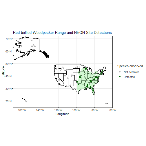
At this broad scale, this estimate is mostly descriptive and could be approximated directly from the data. Occupancy estimates become more informative when applied at finer spatial scales or when combined with covariates, which help explain why species occurs in some locations but not others.
The estimated detection probability (p) is about 0.86, meaning that if the species is present at a site, there is about a 86% chance it will be detected.
Comparing Species
Now that we have demonstrated a simple occupancy model, we can repeat the same workflow for additional species and compare their occupancy and detection probabilities.
Below we fit the same model for:
- Bubo virginianus (Great Horned Owl)
- Cyanocitta cristata (Blue Jay)
For each species, we construct a detection history, create a pao object, and fit the same simple occupancy model (psi ~ 1, p ~ 1), following the same steps as above.
# Function to run the simple occupancy model workflow for any species

run_simple_species_model <- function(species_name, common_name){

  brd_species <- brd_joineddata_clean %>%
    filter(siteID %in% sites,
           scientificName == species_name)

  detections <- brd_species %>%
    group_by(siteID, year) %>%
    summarize(present = 1, .groups = "drop")

  detection_history <- valid_site_years %>%
    left_join(detections, by = c("siteID", "year")) %>%
    mutate(present = replace_na(present, 0)) %>%
    pivot_wider(names_from = year, values_from = present) %>%
    arrange(siteID) %>%
    select(siteID, sort(names(.)[-1]))

  pao <- createPao(
    data = detection_history[, -1],
    unitnames = detection_history$siteID,
    title = common_name
  )

  model <- occMod(
    data = pao,
    model = list(
      psi ~ 1,
      p ~ 1
    ),
    type = "so"
  )

  return(model)
}
Now we run the model for both species.
owl_model <- run_simple_species_model(
  species_name = "Bubo virginianus",
  common_name = "Great Horned Owl"
)


jay_model <- run_simple_species_model(
  species_name = "Cyanocitta cristata",
  common_name = "Blue Jay"
)
Next, we extract the estimated occupancy (ψ) and detection probability (p) for each species.
# Function to extract and rename estimates for simple model

extract_estimates <- function(model){

  ests <- as.data.frame(print_one_site_estimates(mod = model))

  ests <- ests[1:2,] %>%
    mutate(Parameter = c("psi", "p")) %>%
    select(Parameter, est, se, lower, upper) %>%
    rename(
      Estimate = est,
      SE = se,
      L95 = lower,
      U95 = upper
    )

  return(ests)
}


owl_estimates <- extract_estimates(owl_model) %>%
  mutate(Species = "Great Horned Owl")


jay_estimates <- extract_estimates(jay_model) %>%
  mutate(Species = "Blue Jay")


# Combine estimates for plotting

species_estimates <- bind_rows(owl_estimates, jay_estimates)
We'll visualize the estimates in a plot.
ggplot(species_estimates,
       aes(x = Parameter, y = Estimate, fill = Species)) +
  geom_col(position = position_dodge(width = 0.7), width = 0.6) +
  geom_errorbar(aes(ymin = L95, ymax = U95),
                position = position_dodge(width = 0.7),
                width = 0.15) +
  scale_x_discrete(
    limits = c("psi", "p"),
    labels = c(
      psi = "Occupancy (ψ)",
      p = "Detection (p)"
    )
  ) +
  scale_y_continuous(limits = c(0, 1)) +
  labs(
    x = NULL,
    y = "Estimated Probability",
    title = "Occupancy and Detection Estimates by Species"
  ) +
  theme_bw()
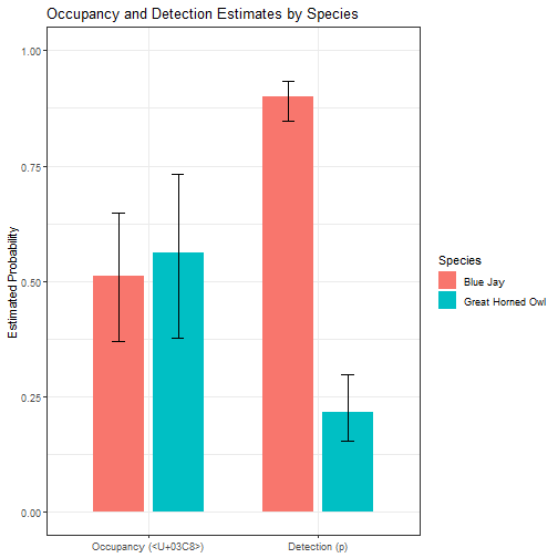
Here we can see that although Blue Jays and Great Horned Owls have similar occupancy probabilities (.51 and .56), their detection probabilities differ dramatically (.90 and .22). Blue Jays are highly detectable during point-count surveys, whereas Great Horned Owls are much more difficult to detect under the same protocol.
Introducing Covariates
In reality, occupancy and detection probabilities are rarely constant across all sites and surveys. Many factors can influence whether a species occurs at a site and whether it is detected during a survey. These factors can be included in occupancy models as covariates.
Site characteristics can influence occupancy or detection. For example:
- Vegetation density – dense vegetation may make birds harder to detect than in more open habitats.
- Habitat type – some species only occupy sites with suitable habitat, such as forests, wetlands, or grasslands.
Survey characteristics can only affect detection. For example:
- Observer differences – some observers may be better at detecting or identifying certain species.
- Weather conditions – rain, wind, or poor visibility can make birds harder to hear or see.
By including these variables in our model, we can either:
- Account for known sources of variation to improve model fit or
- Test whether occupancy or detection is dependent on a particular covariate.
Site Covariates
So far, our model assumed that occupancy and detection probabilities were constant across all sites and surveys. Site characteristics often influence whether a species occupies a location or is more easily detected. We can test these effects by including site covariates in the occupancy model. Remember that site characteristics can influence both occupancy and/or detection.
In this example, we examine if elevation influences the occupancy probability of Melanerpes carolinus (Red-bellied Woodpecker).
Create a site covariate table
Site-level covariates must be provided to createPao() as a separate table with one row per site. The rows must correspond to the same sites used in the detection history.
Here we extract the elevation for each site from the combined dataset brd_joineddata_clean we prepared at the beginning of the tutorial.
site_cov <- brd_joineddata_clean %>%
  select(siteID, elevation) %>%
  distinct(siteID, .keep_all = TRUE) %>%
  arrange(siteID) %>%
  tibble::column_to_rownames("siteID")


head(site_cov, n=10)

##      elevation
## ABBY     386.6
## BARR       5.6
## BART     297.2
## BLAN     137.4
## BONA     403.6
## CLBJ     312.5
## CPER    1637.1
## DCFS     590.4
## DEJU     453.3
## DELA      23.7
Note that other types of site covariates could also be used. For example, categorical variables such as land cover class could be included instead. When including categorical variables as covariates, they must be converted to factors.
# Example categorical covariate

 site_cov_categorical <- brd_perpoint_clean %>%
   select(siteID, nlcdClass) %>%
   distinct(siteID, .keep_all = TRUE) %>%
   mutate(nlcdClass = as.factor(nlcdClass)) %>%
   arrange(siteID) %>%
   tibble::column_to_rownames("siteID")


site_cov_categorical$nlcdClass <- factor(site_cov_categorical$nlcdClass)


head(site_cov_categorical, n=10)

##                       nlcdClass
## ABBY        grasslandHerbaceous
## BARR emergentHerbaceousWetlands
## BART                mixedForest
## BLAN            deciduousForest
## BONA                 shrubScrub
## CLBJ            deciduousForest
## CPER        grasslandHerbaceous
## DCFS        grasslandHerbaceous
## DEJU                 shrubScrub
## DELA              woodyWetlands
Create the Presence-Absence Object (pao)
Next, we create a new pao object that includes the site covariate table. We will use the same detection_history table as before.
birds_pao_sitecov <- createPao(
  data = detection_history[, -1], # detection/nondetection data (survey columns only) from detection_history
  unitnames = detection_history$siteID, # site IDs from detection_history
  unitcov = site_cov # add the site covariates
)
Fit the covariate model
We now fit a model where occupancy varies with elevation, while detection probability remains constant.
In this model, the formula psi ~ elevation specifies that occupancy probability is modeled as a linear function of elevation, meaning the model estimates how occupancy probability changes as elevation increases or decreases. As a result, occupancy probability will not be a single value but will vary depending on the elevation of each site.
Other functional forms can also be used, but aren't included in this tutorial. For example:
-
psi ~ elevation + I(elevation^2)could model a polynomial relationship. For example, a species might prefer mid-elevation forests but be less common at both low and high elevations. -
psi ~ elevation + forest_covercould include multiple covariates influencing occupancy. For example, a bird may be more likely to occur at higher elevations and in areas with greater forest cover. -
psi ~ elevation * forest_covercould model an interaction between variables. For example, forest cover might increase occupancy at low elevations but have little effect at high elevations.
Detection probability could also be modeled as a function of site covariates in the same way. In this example, however, we keep detection probability constant using p ~ 1 so that we can focus on how elevation influences occupancy.
birds_occupancy_sitecov <- occMod(
  data = birds_pao_sitecov,
  model = list(psi ~ elevation,
               p ~ 1),
  type = 'so'
  )
Model Results
Now that the model has been fit, we can examine the results to see whether elevation improves model performance and how it influences occupancy probability. We will do this by:
- Comparing AIC values to evaluate which model provides the best balance between model fit and complexity.
- Calculating a likelihood ratio test to determine whether adding the elevation covariate significantly improves model fit.
- Inspecting the model coefficients to understand the direction and strength of the relationship between elevation and occupancy probability.
- Visualizing the predicted occupancy values to illustrate how occupancy probability changes across the elevation gradient.
Compare AIC (Akaike Information Criterion)
We can compare the new model with elevation to the original model without to see whether including elevation improves the model fit. One common way to compare models is using AIC (Akaike Information Criterion), which balances model fit with model complexity. In general, models with lower AIC values are preferred.
The output table also includes additional statistics, such as the −2 log-likelihood (neg2ll) and other model parameters. These metrics can also be used to evaluate model performance, but we will focus on AIC for this tutorial.
mod.list <-  list(
    birds_occupancy_simple, # the model with formula psi ~ 1, p ~ 1
    birds_occupancy_sitecov # the model with formula psi ~ elevation, p ~ 1
)

aictable <- createAicTable(mod.list = mod.list)

aictable$table

##                Model      AIC   neg2ll npar warn.conv warn.VC    DAIC modlike    wgt
## 2 psi(elevation)p(1) 191.7794 185.7794    3         7       0  0.0000   1e+00 0.9997
## 1         psi(1)p(1) 207.9761 203.9761    2         7       0 16.1967   3e-04 0.0003
Looking at the two models, the model including elevation has a lower AIC value (191.7794 vs 207.9761). Because AIC balances model fit with the number of parameters, the lower value suggests that the model including elevation provides a better and more parsimonious explanation of the data.
Likelihood Ratio Test
We can also calculate a p-value using a likelihood ratio test (LRT) to quantify whether the model including elevation provides a significantly better fit than the simpler model without it. This method is appropriate for “nested” models only, meaning the simpler model is a special case of the more complex one. In this case, the simple model (psi ~ 1) is a reduced version of the model that includes elevation (psi ~ elevation).
The likelihood ratio test compares how well the two models explain the data by examining the difference in their −2 log-likelihood values. The difference in −2 log-likelihood values is compared to a chi-square distribution, where the degrees of freedom equals the difference in the number of parameters between the two models.
#get the difference in the neg2loglike between the two models

diff <- abs(birds_occupancy_simple$neg2loglike - birds_occupancy_sitecov$neg2loglike)


#look up our observed difference on a chi-square distribution with 1 degree of freedom (the difference between the number of parameters)

pchisq(diff,
       df = abs(birds_occupancy_simple$npar - birds_occupancy_sitecov$npar),
       lower.tail = FALSE)

## [1] 1.992237e-05
The resulting p-value tests the null hypothesis that adding elevation does not improve the model fit. Because the p-value is very small (1.992237e-05), we reject the null hypothesis and conclude that including elevation significantly improves the model. Therefore, elevation appears to be an important predictor of occupancy for this species in our dataset!
Inspect coeffiecients
We can also examine the estimated coefficients from the model to understand exactly how the covariate influences occupancy probability. In this case, the coefficient for elevation tells us the direction and strength of the relationship between elevation and the probability that a site is occupied.
coef(birds_occupancy_sitecov, 'psi', prob = 0.95)

##                           Beta_est       se      lowerCI      upperCI
## psi_A1.Int                1.477853 0.378737  0.735542120  2.220163880
## psi_A1.Int.psi.elevation -0.002936 0.000668 -0.004245256 -0.001626744
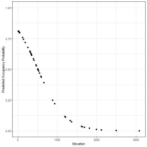
The beta estimate for elevation is slightly negative (-0.002936), meaning that occupancy probability decreases as elevation increases.
The output also includes 95% confidence intervals for each estimate. In this case, the confidence interval for elevation (-0.004245256 to -0.001626744) does not include 0 and lies entirely below it. This indicates that the estimated relationship between elevation and occupancy is consistently negative across the range of plausible values for the coefficient. In other words, it is quite likely that occupancy probability decreases as elevation increases.
Display Results
It can also be helpful to visually examine how occupancy probability changes across the elevation gradient. To do this, we extract the predicted occupancy probabilities for each site from the model output and plot them against site elevation.
data <- cbind(site_cov, birds_occupancy_sitecov$real$psi) %>%
  distinct(.keep_all = TRUE) %>%
  arrange(elevation)


ggplot(data, aes(x = elevation, y = est)) +
  geom_point(size = 2, alpha = 0.8) +
  labs(
    x = "Elevation",
    y = "Predicted Occupancy Probability"
  ) +
  scale_y_continuous(limits = c(0, 1)) +
  theme_bw()
Survey Covariates
In addition to site characteristics, the conditions under which a survey is conducted can also influence whether a species is detected. Factors such as weather, time of day, or observer differences can affect how likely it is that an observer detects a species during a survey.
Unlike site covariates, survey covariate can only influence detection probability, not whether a species occupies a site.
In this example, we examine whether survey effort influences the detection probability of Melanerpes carolinus. Survey effort here is defined as the total number of minutes spent conducting bird point-count surveys at a site within a year. Although each survey lasts six minutes, the number of surveys conducted can vary among site–year combinations due to differences in sampling design (e.g., large vs. small sites) and the number of plots sampled at each site. Greater survey effort could provide more opportunities to detect a species if it is present.
Create a survey covariate table
NEON bird surveys follow a standardized protocol in which each point-count survey lasts 6 minutes. To estimate survey effort for each site–year combination, we count the number of point-count surveys conducted and multiply by six minutes. Survey covariates supplied to createPao() must be provided in the same order as the rows and columns of detection_history, so we also sort by siteID and year to match.
survey_effort <- brd_perpoint_clean %>% # we start with brd_perpoint_clean since we want all point-count surveys conducted, not just those that detected birds
  distinct(pointSurveyID, siteID, year) %>%
  group_by(siteID, year) %>%
  summarize(
    survey_effort = n() * 6, # the number of surveys multiplied by 6
    .groups = "drop"
  ) %>%
  pivot_wider(
    names_from = year,
    values_from = survey_effort,
    values_fill = 0 # We can fill in NAs as 0s since no time was spend conducting surveys for incomplete surveys
  ) %>%
  tibble::column_to_rownames("siteID") %>% # sort siteIDs alphabetically
  select(sort(names(.))) # sort years


head(survey_effort, n=10)

##      2017 2018 2019 2020 2021 2022 2023 2024
## ABBY  258  156  240    0  228  228  228  204
## BARR  432  426  426    0  378  318  378  378
## BART  474  474  468  474  480  474  480  480
## BLAN  144  132  120  132  132  132  132  132
## BONA  810  522  540  534  540  540  534  540
## CLBJ  486  486  486  480  486  486  486  486
## CPER  810  540  540  540  540  540  540  540
## DCFS  240  240  240  240  240  240    0  240
## DEJU  540  540  540  540  540  540  540  540
## DELA  216  180  180  168  168  168  168  168
createPao() expects survey covariates in a single column vector rather than a matrix, so we flatten the survey_effort matrix into a vector.
# flatten the data frame

surveycov <-  data.frame(
  survey_effort = unlist(survey_effort)
  #it is possible to add other survey covariates here
  )


# remove the rownames

row.names(surveycov) <- NULL


head(surveycov)

##   survey_effort
## 1           258
## 2           432
## 3           474
## 4           144
## 5           810
## 6           486
Create the Presence-Absence Object (pao)
Next we create a new pao object that includes both the site covariate (elevation) from before (since adding elevation provides a better model fit) and the survey covariate (survey effort).
birds_pao_surveycov <- createPao(
  data = detection_history[, -1], # detection/nondetection data (survey columns only) from detection_history
  unitnames = detection_history$siteID, # site IDs from detection_history
  unitcov = site_cov, # add the site covariates
  survcov = surveycov # add the survey covariates
)
Fit the covariate model
We now fit a model where:
- occupancy varies linearly with elevation
- detection probability varies linearly with survey effort
Let's see if this is a better fit.
birds_occupancy_surveycov <- occMod(
  data = birds_pao_surveycov,
  model = list(psi ~ elevation,  p ~ survey_effort),
  type = 'so'
  )


summary(birds_occupancy_surveycov)

## Model name=psi(elevation)p(survey_effort)
## AIC=193.1907
## -2*log-likelihood=185.1907
## num. par=4
## Warning: Numerical convergence may not have been reached. Parameter estimates converged to approximately 7 signifcant digits.
Model Results
We can evaluate the survey covariate model using the same approaches used above.
Compare AIC (Akaike Information Criterion)
We can again compare models using AIC. Here we compare the simple original model, the site covariate elevation model, and the survey covariate survey_effort model.
mod.list <-  list(
    birds_occupancy_simple, # the model with formula psi ~ 1, p ~ 1
    birds_occupancy_sitecov, # the model with formula psi ~ elevation, p ~ 1
    birds_occupancy_surveycov # the model with formula psi ~ elevation, p ~ survey_effort
)

aictable <- createAicTable(mod.list = mod.list)

aictable$table

##                            Model      AIC   neg2ll npar warn.conv warn.VC    DAIC modlike
## 2             psi(elevation)p(1) 191.7794 185.7794    3         7       0  0.0000  1.0000
## 3 psi(elevation)p(survey_effort) 193.1907 185.1907    4         7       0  1.4113  0.4938
## 1                     psi(1)p(1) 207.9761 203.9761    2         7       0 16.1967  0.0003
##      wgt
## 2 0.6693
## 3 0.3305
## 1 0.0002
Looking at the three models, the model including elevation only has the lowest AIC value (191.7794), followed by the model including elevation and survey effort (193.1907), and finally the simple model with no covariates (207.9761). This suggests that adding survey effort as a detection covariate does not improve the model relative to the elevation-only model, and the additional parameter does not provide enough improvement in model fit to justify the more complex model.
Likelihood Ratio Test
We can also calculate a p-value using a likelihood ratio test to quantify whether adding survey effort improves the model relative to the elevation-only model. Remember, we can do this because the psi ~ elevation, p ~ 1 model is a simpler version of the psi ~ elevation, p ~ survey_effort model.
#get the difference in the neg2loglike between the two models

diff <- abs(birds_occupancy_sitecov$neg2loglike - birds_occupancy_surveycov$neg2loglike)


#look up our observed difference on a chi-square distribution with 1 degree of freedom (the difference between the number of parameters)

pchisq(diff,
       df = abs(birds_occupancy_sitecov$npar - birds_occupancy_surveycov$npar),
       lower.tail = FALSE)

## [1] 0.4429223
The resulting p-value tests the null hypothesis that including survey effort does not improve the model fit. In this case, the p-value (0.4429223) is relatively large, meaning we do not have evidence that adding survey effort improves the model.
Inspect coeffiecients
Lets take a look at the coeffients associated with our model.
coef(birds_occupancy_surveycov, 'p', prob = 0.95)

##                            Beta_est       se      lowerCI      upperCI
## p1_B1.Int                  2.279714 0.332403  1.628216092 2.9312119084
## p1_B1.Int.p.survey_effort -0.001102 0.000728 -0.002528854 0.0003248538
The coefficient for survey effort is slightly negative (-0.001102), meaning the model estimates that detection probability decreases slightly as survey effort increases. However, the 95% confidence interval for this estimate (-0.00253 to 0.00032) includes 0. This means the data are consistent with either a small negative effect, no effect, or even a very small positive effect. In other words, the coefficient estimates do not provide strong evidence that survey effort meaningfully influences detection probability either.
Display Results
Finally, we can visualize how predicted detection probability changes across the range of survey effort values, just to see what it looks like, even though we are fairly confident that survey_effort does not have any real effect on detection for Melanerpes carolinus.
data <- cbind(surveycov, birds_occupancy_surveycov$real$p) %>%
  distinct(.keep_all = TRUE) %>%
  arrange(survey_effort)


ggplot(data, aes(x = survey_effort, y = est)) +
  geom_point(size = 2, alpha = 0.8) +
  labs(
    x = "Survey Effort",
    y = "Predicted Detection Probability"
  ) +
  scale_y_continuous(limits = c(0, 1)) +
  theme_bw()
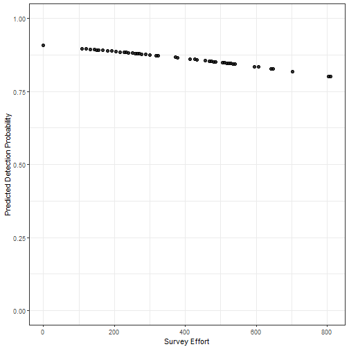
Biologically, the fact that survey_effort does not have any real effect on detection likely has to do with Melanerpes carolinus's high detection rate (80%-90%). Since the species is already highly detectable, observers are likely to detect it quickly when it is present, so increasing survey effort does not meaningfully increase detection probability.
Conclusion
In this tutorial, we demonstrated how NEON breeding landbird data can be used to build detection histories and fit a single-species, single-season occupancy model. We estimated occupancy and detection probabilities, incorporated both site-level and survey-level covariates and examined ways to test model performance.
While this tutorial focused on a relatively simple, but powerful, model, occupancy modeling can be extended in several ways. For example, multi-season occupancy models allow occupancy probability to change over time (we assumed it was constant here), enabling researchers to estimate local colonization and extinction rates and their predictors for a species. Multi-species occupancy models can also be used to analyze patterns across entire communities at a location, allowing researchers to examine how species traits influence occupancy and detection probabilities.