Plot spectral signatures of AOP Reflectance data in GEE

Read in the AOP Directional Reflectance Image

As should be familiar by now from the previous tutorials in this series, we'll start by pulling in the AOP data. For this exercise we will only read directional reflectance data from SOAP collected in 2021:

// Filter image collection by date and site
var soapSDR = ee.ImageCollection("projects/neon-prod-earthengine/assets/HSI_REFL/001")
  .filterDate('2021-01-01', '2021-12-31')
  .filterMetadata('NEON_SITE', 'equals', 'SOAP')
  .first();

// Create a 3-band true-color image 
var soapSDR_RGB = soapSDR.select(['B053', 'B035', 'B019']);

// Display the SDR image
Map.addLayer(soapSDR_RGB, {min:103, max:1160}, 'SOAP 2021 Reflectance RGB');

// Center the map around the soapSDR_RGB object, set zoom to 12
Map.centerObject(soapSDR_RGB, 12);

Extract data bands

Next we will extract only the "data" bands in order to plot the spectral information. The reflectance data contains 426 data bands, and a number of QA/Metdata bands that provide additional information that can be useful in interpreting and analyzing the data (such as the Weather Quality Information). For plotting the spectra, we only need the data bands.

// Pull out only the data bands (these all start with B, eg. B001)
var soapSDR_data = soapSDR.select('B.*')
print('SOAP SDR Data',soapSDR_data)

// Read in the properties as a dictionary
var properties = soapSDR.toDictionary()

Extract wavelength information from the properties

Similar to the code above, we can use a regular expression to pull out the wavelength information from the properties. The wavelength and Full Width Half Max (FWHM) information is stored in the properties starting with WL_FWHM_B. These are stored as strings, so the nex step is to write a funciton that converts the string to a float, and only pulls out the center wavelength value (by splitting on the "," and pulling out only the first value). This is all we need for now, but if you needed the FWHM information, you could write a similar function. Lastly, we'll apply the function using GEE .map to pull out the wavelength information. We an then print some information about what we've extracted

// Select the WL_FWHM_B*** band properties (using regex)
var wl_fwhm_dict = properties.select(['WL_FWHM_B+\\d{3}']);

// Pull out the wavelength, fwhm values to a list
var wl_fwhm_list = wl_fwhm_dict.values()
print('Wavelength FWHM list:',wl_fwhm_list)

// Function to pull out the wavelength values only and convert the string to float
var get_wavelengths = function(x) {
  var str_split = ee.String(x).split(',')
  var first_elem = ee.Number.parse((str_split.get(0)))
  return first_elem
}

// apply the function to the wavelength full-width-half-max list
var wavelengths = wl_fwhm_list.map(get_wavelengths)

print('Wavelengths:',wavelengths)
print('# of data bands:',wavelengths.length())

Interactively plot the spectral signature of a pixel

Lastly, we'll create a plot in the Map panel, and use the Map.onClick function to create a spectral signature of a given pixel that you click on. Most of the code below specifies formatting, figure labels, etc.

// Create a panel to hold the spectral signature plot
var panel = ui.Panel();
panel.style().set({width: '600px',height: '300px',position: 'top-left'});
Map.add(panel);
Map.style().set('cursor', 'crosshair');

// Create a function to draw a chart when a user clicks on the map.
Map.onClick(function(coords) {
  panel.clear();
  var point = ee.Geometry.Point(coords.lon, coords.lat);
    wavelengths.evaluate(function(wvlnghts) {
      var chart = ui.Chart.image.regions({
        image: soapSDR_data, 
        regions: point, 
        scale: 1,
        seriesProperty: 'λ (nm)', 
        xLabels: wavelengths.getInfo()
    });
    chart.setOptions({
      title: 'Reflectance',
      hAxis: {title: 'Wavelength (nm)', 
      vAxis: {title: 'Reflectance'},
      gridlines: { count: 5 }}
    });
    // Create and update the location label 
    var location = 'Longitude: ' + coords.lon.toFixed(2) + ' ' +
                   'Latitude: ' + coords.lat.toFixed(2);
    panel.widgets().set(1, ui.Label(location));
    panel.add(chart);
  })
});

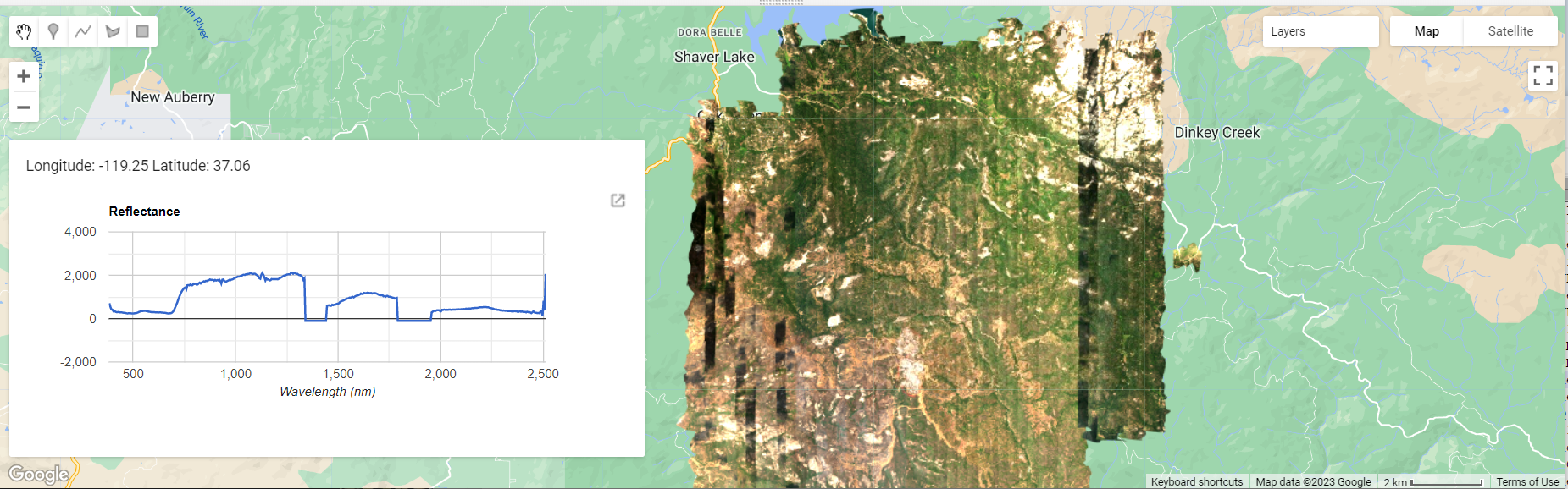
When you run this code (linked at the bottom), you will see the SOAP 2021 directional reflectance layer show up in the Map panel, along with an empty white figure panel in the lower left corner. When you click anywhere in the reflectance image, the empty figure panel will be populated with the spectral signature of the pixel you clicked on.

QA Considerations - Bad and Noisy Bands

Let's zoom in on the spectral signature figure to take a closer look. Specifically, you can easily spot some QA considerations that are important to factor in if you intend to work with all 426 bands of data.

Water Vapor Band Windows

We can see from the spectral profile above that the reflectance values dip to below zero around ~1400 nm and ~1800 nm. These are water vapor band windows, resulting from water vapor which absorbs light between wavelengths 1340-1445 nm and 1790-1955 nm. The atmospheric correction that converts radiance to reflectance subsequently results in a spike at these two bands, and are invalid values. They are set to -100 for the reflectance data in GEE. For more details on these bands, please refer to the Plot a Spectral Signature from Reflectance Data in Python tutorial. If you are working with hyperspectral data downloaded from the NEON Data Portal, these water vapor band windows are not set to -100, so this is one difference between the reflectance datasets on GEE and the datasets and the original hdf5 reflectance datasets.

Noisy Bands

You may also notice that the reflectance values the beginning (~380 nm) and end (~2500 nm) of the wavelength range spike up, relative to the other nearby bands. These are not a feature of the actual data. The first and last bands are more prone to have noisy values due to imperfect calibration of the sensor at the lowest and highest reflectance bands. Best practice is to leave out the first and last 5-10 bands of data; you can inspect a spectral signature plot to determine how many bands to remove.

Recap

In this lesson you learned how to read in wavelength information from the Surface Directional Reflectance properties in GEE, created functions to convert from one data format to another, and created an interactive plot to visualize the spectral signature of a selected pixel. You can quickly see how GEE is a powerful tool for interactive data visualization and exploratory analysis.

Get Lesson Code

AOP GEE Reflectance Plot Spectra