NDVI Time Series using AOP Reflectance and Landsat 8 Data in GEE

In this lesson, we'll continue to use the Great Smokey Mountains site as an example, this time creating a time series of the mean NDVI within the Chimney Tops 2 Fire perimeter between 2016-2022. We will plot this along with the NDVI time-series derived from Landsat 8 data, and use this to fill in some more detailed temporal information.

AOP strives to collect every site during peak-greenness, when the predominant vegetation is most photosynthetically active. This is so that when comparing data from year to year, the differences are due to actual changes and not just due to the time of year. This is not always possible, so it's important to consider the time of year when you are conducting your analysis.

Read in AOP and Landsat 8 Surface Reflectance Image Collections

First read in the AOP directional reflectance data and the Landsat 8 data, filtering the AOP data by the site (GRSM) and filtering the Landsat data by the Chimney Tops Fire region of interest, and by date.

// Specify center location for GRSM
// Site lat/lon can be found on the field site page: https://www.neonscience.org/field-sites/grsm
var site_center = ee.Geometry.Point([-83.5, 35.7]); 

// Create region of interest (roi)
var roi = ee.FeatureCollection('projects/neon-sandbox-dataflow-ee/assets/chimney_tops_fire')

// Read in the reflectance Image Collection
var sdr_col = ee.ImageCollection('projects/neon-prod-earthengine/assets/HSI_REFL/001')
  .filterMetadata('NEON_SITE', 'equals', 'GRSM')

// Read in Landsat 8 Surface Reflectance Image Collection
var l8sr = ee.ImageCollection('LANDSAT/LC08/C02/T1_L2')
                .filterBounds(roi)
                .filter(ee.Filter.calendarRange(2016, 2022, 'year'));

Cloud Mask Function for Landsat 8 Data

Next we can create a function to pre-process the Landsat 8 data, which applies scaling and cloud / saturated data masking. Don't worry too much about the details here, but the main thing to be aware of is that different satellite image collections handle the QA information differently. Landsat (and other satellites) often use something called "bitmasking" to store QA information, which is a space-efficient storage method. This cloud-masking function can be found on the earthengine-api GitHub examples here.

// cloud masking function for Landsat 8 Collection 2 
function maskL8sr(image) {

  var qaMask = image.select('QA_PIXEL').bitwiseAnd(parseInt('11111', 2)).eq(0);
  var saturationMask = image.select('QA_RADSAT').eq(0);

  // Apply the scaling factors to the appropriate bands.
  var opticalBands = image.select('SR_B.').multiply(0.0000275).add(-0.2);
  var thermalBands = image.select('ST_B.*').multiply(0.00341802).add(149.0);

  // Replace the original bands with the scaled ones and apply the masks.
  return image.addBands(opticalBands, null, true)
      .addBands(thermalBands, null, true)
      .updateMask(qaMask)
      .updateMask(saturationMask);
}

// Apply the cloud masking function
l8sr = l8sr.filterBounds(roi).map(maskL8sr)

Merge AOP and Landsat 8 NDVI Collections

Next we can plot the two datasets on the same chart. This code was modified from this Stack Overflow post.

// compute ndvi bands to add to each collection
var addL8Bands = function(image){
  var l8_ndvi = image.normalizedDifference(['SR_B5','SR_B4']).rename('l8_ndvi')
  var aop_ndvi = ee.Image().rename('aop_ndvi') 
  return image.addBands(l8_ndvi).addBands(aop_ndvi)
}

var addAOPBands = function(image){
  var aop_ndvi = image.normalizedDifference(['B097', 'B055']).rename('aop_ndvi')
  var l8_ndvi = ee.Image().rename('l8_ndvi') 
  return image.addBands(aop_ndvi).addBands(l8_ndvi)
}

l8sr = l8sr.map(addL8Bands)
sdr_col = sdr_col.map(addAOPBands)

print('NIS Images',sdr_col)

// merge the collections
var merged = l8sr.merge(sdr_col).select(['l8_ndvi', 'aop_ndvi'])

Plot NDVI Time Series

Lastly we can create and plot (print) the time-series chart. Most of this is just setting the chart style.

// Set chart style properties.
// https://developers.google.com/earth-engine/guides/charts_style
var chartStyle = {
  title: 'NDVI at Chimney Tops Fire ROI - AOP + Landsat 8',
  hAxis: {
    title: 'Date',
    titleTextStyle: {italic: false, bold: true},
    gridlines: {color: 'FFFFFF'}
  },
  vAxis: {
    title: 'Mean NDVI',
    titleTextStyle: {italic: false, bold: true},
    gridlines: {color: 'FFFFFF'},
    format: 'short',
    baselineColor: 'FFFFFF'
  },
  series: {
    0: {lineWidth: 3, color: 'E37D05', pointSize: 7},
    1: {lineWidth: 3, color: '1D6B99'}
  },
  chartArea: {backgroundColor: 'EBEBEB'}
};

// Plot the merged (AOP + Landsat 8) Image Collection NDVI Time Series
var ndvi_timeseries = ui.Chart.image.series({
  imageCollection: merged,
  region: roi,
  reducer: ee.Reducer.mean(),
  scale: 30 // 	Scale to use with the reducer in meters
}).setOptions(chartStyle);

print(ndvi_timeseries)

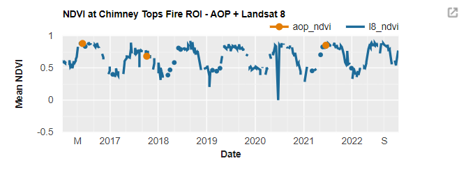
This figure demonstrates some important points. First, we can see that there is fairly good alignment between the mean NDVI calculated from AOP reflectance data and Landsat 8 at these times. While the Airborne Observation Platform seeks to collect data in peak green conditions, this is not always possible due to logistical or other constraints. For this site, one of the AOP collections in 2017 was in October, past peak-greenness, and the leaves already started senescing in some areas. Generating a time-series plot like this can help highlight the data in the context of the larger temporal trends. In this example, the NDVI time-series generated from Landsat 8 shows strong seasonal trends, as you might expect. This brings us to the second point: while AOP data has very high spectral (426 bands) and spatial (1m) resolution, the temporal resolution (site visits 3 out of every 5 years) may not provide enough temporal coverage, depending on your research application. This is where scaling with satellite data - either to expand your analysis to a larger area, or to achieve a more comprehensive temporal picture - can be useful. This tutorial demonstrates a simple example of scaling with satellite data to fill in temporal resolution for a basic NDVI calculation, and shows how GEE makes this sort of scalable analysis much simpler!

Get Lesson Code

GRSM NDVI Time Series - Landsat 8 & AOP