Plot NEON RGB Camera Imagery in Python

This tutorial introduces NEON's Level 3 (mosaicked) RGB camera images, Data Product (DP3.30010.001) and uses the Python package rasterio to read in and plot the camera data in Python. In this lesson, we will read in an RGB camera tile collected over the NEON Smithsonian Environmental Research Center (SERC) site and plot the mutliband image, as well as the individual bands. This lesson was adapted from the rasterio plotting documentation.

Background

As part of the NEON Airborne Operation Platform's suite of remote sensing instruments, the digital camera produces high-resolution (<= 10 cm) photographs of the earth’s surface. The camera records light energy that has reflected off the ground in the visible portion (red, green and blue) of the electromagnetic spectrum. Often the camera images are used to provide context for the hyperspectral and LiDAR data, but they can also be used for research purposes in their own right. One such example is the tree-crown mapping work by Weinstein et al. - see the links below for more information!

• Individual Tree-Crown Detection in RGB Imagery Using Semi-Supervised Deep Learning Neural Networks
• A remote sensing derived data set of 100 million individual tree crowns for the National Ecological Observatory Network
• DeepForest: A Python package for RGB deep learning tree crown delineation

For more interactive notebooks showing examples of working with airborne camera imagery, including with the DeepForest package (and other environmental applications), check out:

• Environmental Data Science (EDS) Book and the EDS Notebook Gallery

In this lesson we will keep it simple and show how to read in and plot a single camera file (1km x 1km ortho-mosaicked tile) - a first step in any research incorporating the AOP camera data (in Python).

Tip: To run a code chunk (cell) in Jupyter Notebook you can either select Cell > Run Cells with your cursor placed in the cell you want to run, or use the shortcut key Shift + Enter. For more handy shortcuts, refer to the tab Help > Keyboard Shortcuts.

Import required packages

First let's import the packages that we'll be using in this lesson.

import os
import dotenv
import neonutilities as nu
import rasterio as rio
from rasterio.plot import show, show_hist
import matplotlib.pyplot as plt

Next, let's download a single camera file (1 km x 1 km tile).

As of June 2026, NEON requires an API token for data downloads, to reduce bot scraping and improve user support. Tokens can be generated in NEON data portal user accounts - log in to your account or create one, and go to the API Tokens section. For best practices in storing and using tokens, follow the instructions here. Once you've set up your token as an environment variable, you can load it using the python-dotenv package as follows, optionally specifying the path to the .env file in load_dotenv().

dotenv.load_dotenv()
token = os.environ.get("NEON_TOKEN")

# download the RGB Camera data to the C:/data directory - change this if desired
nu.by_tile_aop(dpid='DP3.30010.001',
               site='SERC',
               year=2021,
               easting=368000,
               northing=4306000,
               token=token,
               savepath=r'C:\data')

Provisional NEON data are not included. To download provisional data, use input parameter include_provisional=True.


Continuing will download 2 NEON data files totaling approximately 68.8 MB. Do you want to proceed? (y/n)  y


Downloading 2 NEON data files totaling approximately 68.8 MB

100%|█████████████████████████████████████████████████████████████████████████████████████████████████████████████████████████| 2/2 [00:01<00:00,  1.05it/s]

Display the RGB tile that you've downloaded:

rgb_dir = os.path.expanduser(r"C:\data\DP3.30010.001")

for root, dirs, files in os.walk(rgb_dir):
    for file in files:
        if file.endswith('.tif'):
            rgb_file = os.path.join(root, file)
            print(rgb_file)

C:\data\DP3.30010.001\neon-aop-products\2021\FullSite\D02\2021_SERC_5\L3\Camera\Mosaic\2021_SERC_5_368000_4306000_image.tif

Open the Camera RGB data with rasterio

We can open and read this RGB data that we downloaded in Python using the rasterio.open function:

# read the RGB file (including the full path) to the variable rgb_dataset
rgb_dataset = rio.open(rgb_file)

Let's look at a few properties of this dataset to get a sense of the information stored in the rasterio object:

print('rgb_dataset:\n',rgb_dataset)
print('\nshape:\n',rgb_dataset.shape)
print('\nspatial extent:\n',rgb_dataset.bounds)
print('\ncoordinate information (crs):\n',rgb_dataset.crs)

rgb_dataset:
 <open DatasetReader name='C:\data\DP3.30010.001\neon-aop-products\2021\FullSite\D02\2021_SERC_5\L3\Camera\Mosaic\2021_SERC_5_368000_4306000_image.tif' mode='r'>

shape:
 (10000, 10000)

spatial extent:
 BoundingBox(left=368000.0, bottom=4306000.0, right=369000.0, top=4307000.0)

coordinate information (crs):
 PROJCS["WGS 84 / UTM zone 18N",GEOGCS["WGS 84",DATUM["World Geodetic System 1984",SPHEROID["WGS 84",6378137,298.257223563]],PRIMEM["Greenwich",0],UNIT["degree",0.0174532925199433,AUTHORITY["EPSG","9122"]]],PROJECTION["Transverse_Mercator"],PARAMETER["latitude_of_origin",0],PARAMETER["central_meridian",-75],PARAMETER["scale_factor",0.9996],PARAMETER["false_easting",500000],PARAMETER["false_northing",0],UNIT["metre",1,AUTHORITY["EPSG","9001"]],AXIS["Easting",EAST],AXIS["Northing",NORTH]]

Unlike the other AOP data products, camera imagery is generated at 10cm resolution, so each 1km x 1km tile will contain 10000 pixels (other 1m resolution data products will have 1000 x 1000 pixels per tile, where each pixel represents 1 meter).

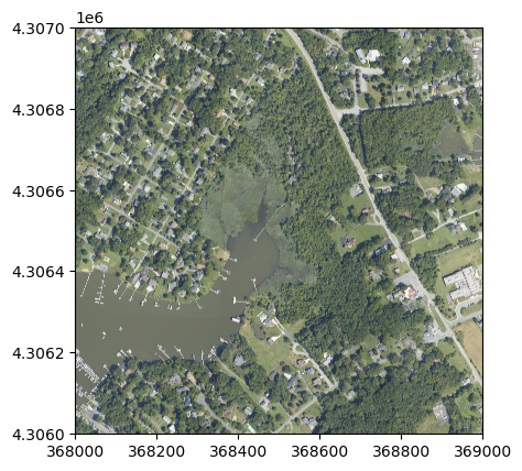
Plot the RGB multiband image

We can use rasterio's built-in functions show to plot the CHM tile.

show(rgb_dataset);

Plot each band of the RGB image

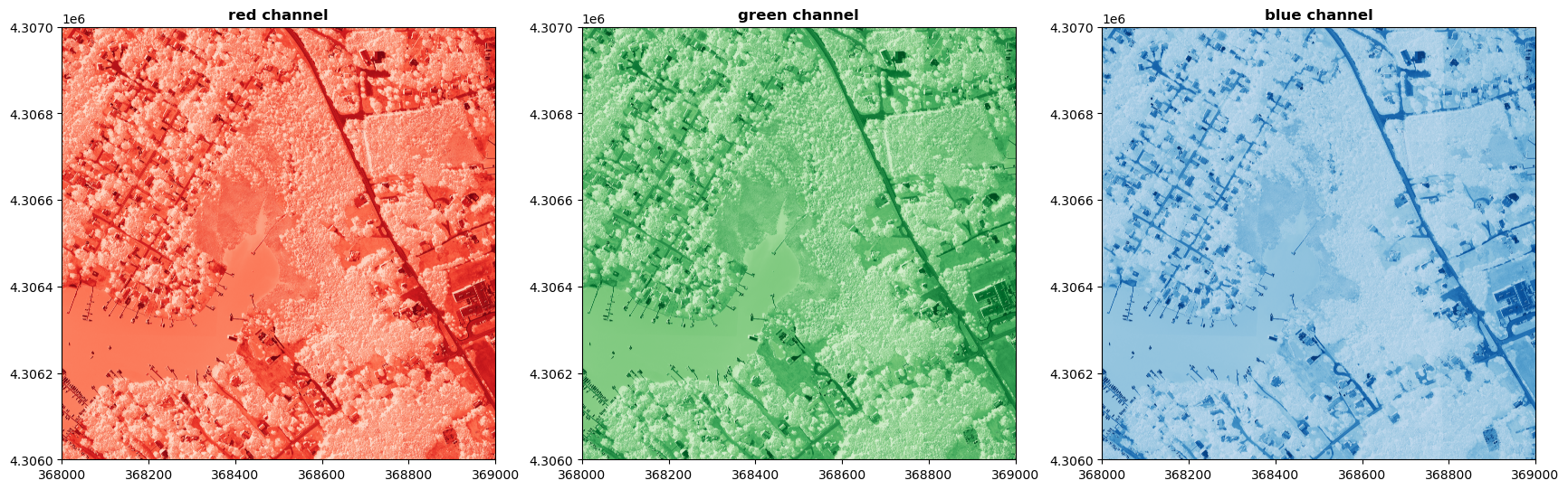
We can also plot each band (red, green, and blue) individually as follows:

fig, (axr, axg, axb) = plt.subplots(1,3, figsize=(21,7))
show((rgb_dataset, 1), ax=axr, cmap='Reds', title='red channel')
show((rgb_dataset, 2), ax=axg, cmap='Greens', title='green channel')
show((rgb_dataset, 3), ax=axb, cmap='Blues', title='blue channel')
plt.show()

That's all for this example! Most of the other AOP raster data are all single band images so you can't make a 3-band composite like for the camera. You can make RGB composites using different bands of the hyperspectral data. In summary, rasterio is a handy Python package for working with any geotiff files. You can download and visualize the lidar and spectrometer derived raster images similarly.