This data tutorial provides an introduction to working with NEON eddy
flux data, using the neonUtilities R package or the
neonutilities Python package. If you are new to NEON data,
we recommend starting with a more general tutorial, such as the
neonUtilities
tutorial or the
Download
and Explore tutorial. Some of the functions and techniques described
in those tutorials will be used here, as well as functions and data
formats that are unique to the eddy flux system.
This tutorial assumes general familiarity with eddy flux data and
associated concepts.
1. Setup and data download
Start by installing and loading packages and setting options.
R
To work with the NEON flux data, we need the rhdf5
package, which is hosted on Bioconductor, and requires a different
installation process than CRAN packages:
The necessary helper packages should be installed automatically when
we install neonUtilities. We’ll also use several modules
that are installed automatically with standard Python installations.
pip install neonutilities
Now load packages.
import neonutilities as nu
import matplotlib.pyplot as plt
import pandas as pd
import numpy as np
from datetime import datetime
import os
Download data
R
Use the zipsByProduct() function from the
neonUtilities package to download flux data from two sites
and two months. The transformations and functions below will work on any
time range and site(s), but two sites and two months allows us to see
all the available functionality while minimizing download size.
Inputs to the zipsByProduct() function for this
tutorial:
dpID: DP4.00200.001, the bundled eddy covariance
product
package: basic (the expanded package is not covered in
this tutorial)
site: NIWO = Niwot Ridge and HARV = Harvard Forest
startdate: 2018-06 (both dates are inclusive)
enddate: 2018-07 (both dates are inclusive)
savepath: path to download to; here we use the working
directory
check.size: T if you want to see file size before
downloading, otherwise F
The download may take a while, especially if you’re on a slow
network. For faster downloads, consider using an
API
token.
Use the zips_by_product() function from the
neonutilities package to download flux data from two sites
and two months. The transformations and functions below will work on any
time range and site(s), but two sites and two months allows us to see
all the available functionality while minimizing download size.
Inputs to the zips_by_product() function for this
tutorial:
dpid: DP4.00200.001, the bundled eddy covariance
product
package: basic (the expanded package is not covered in
this tutorial)
site: NIWO = Niwot Ridge and HARV = Harvard Forest
startdate: 2018-06 (both dates are inclusive)
enddate: 2018-07 (both dates are inclusive)
savepath: path to download to; here we use the working
directory
check_size: T if you want to see file size before
downloading, otherwise F
The download may take a while, especially if you’re on a slow
network. For faster downloads, consider using an
API
token.
There are five levels of data contained in the eddy flux bundle. For
full details, refer to the
NEON
algorithm document.
Briefly, the data levels are:
Level 0’ (dp0p): Calibrated raw observations
Level 1 (dp01): Time-aggregated observations, e.g. 30-minute mean
gas concentrations
Level 2 (dp02): Time-interpolated data, e.g. rate of change of a gas
concentration
Level 3 (dp03): Spatially interpolated data, i.e. vertical
profiles
Level 4 (dp04): Fluxes
The dp0p data are available in the expanded data package and are
beyond the scope of this tutorial.
The dp02 and dp03 data are used in storage calculations, and the dp04
data include both the storage and turbulent components. Since many users
will want to focus on the net flux data, we’ll start there.
3. Extract Level 4 data (Fluxes!)
R
To extract the Level 4 data from the HDF5 files and merge them into a
single table, we’ll use the stackEddy() function from the
neonUtilities package.
stackEddy() requires two inputs:
filepath: Path to a file or folder, which can be any
one of:
A zip file of eddy flux data downloaded from the NEON data
portal
A folder of eddy flux data downloaded by the
zipsByProduct() function
The folder of files resulting from unzipping either of 1 or 2
One or more HDF5 files of NEON eddy flux data
level: dp01-4
Input the filepath you downloaded to using
zipsByProduct() earlier, including the
filestoStack00200 folder created by the function, and
dp04:
The variables and objDesc tables can help
you interpret the column headers in the data table. The
objDesc table contains definitions for many of the terms
used in the eddy flux data product, but it isn’t complete. To get the
terms of interest, we’ll break up the column headers into individual
terms and look for them in the objDesc table:
term <- unlist(strsplit(names(flux$NIWO), split=".", fixed=T))
flux$objDesc[which(flux$objDesc$X...Object %in% term),]
## X...Object
## 22 angZaxsErth
## 84 data
## 91 distReso
## 92 distXaxs90
## 93 distXaxsMax
## 94 distYaxs90
## 95 distZaxsAbl
## 100 distZaxsMeasDisp
## 101 distZaxsRgh
## 125 flux
## 126 fluxCo2
## 128 fluxH2o
## 130 fluxMome
## 132 fluxTemp
## 133 foot
## 200 nsae
## 244 qfFinl
## 274 qfqm
## 451 stat
## 453 stor
## 474 timeBgn
## 475 timeEnd
## 477 turb
## 505 veloFric
## 512 veloYaxsHorSd
## 515 veloZaxsHorSd
## Description
## 22 Wind direction
## 84 Represents data fields
## 91 Resolution of vector of distances (units = m)
## 92 Distance of 90% contriubtion of footprint aligned with dominant wind direction
## 93 Max distance of footprint contriubtion aligned with dominant wind direction
## 94 Distance of 90% contriubtion of footprint aligned with direction that is perpendicular to dominant wind direction
## 95 Atmospheric boundary layer height used in flux footprint calculations
## 100 Measurement height minus displacement height
## 101 Roughness length used in flux footprint calculation
## 125 General term for flux
## 126 CO2 flux (can be turbulent, storage, or nsae)
## 128 H2O flux (can be turbulent, storage, or nsae) - relates to latent heat flux
## 130 Momentum flux (can be turbulent, storage, or nsae)
## 132 Temperature flux (can be turbulent, storage, or nsae) - relates to sensible heat flux
## 133 Footprint
## 200 Net surface atmospher exchange (turbulent + storage fluxes)
## 244 The final quality flag indicating if the data are valid for the given aggregation period (1=fail, 0=pass)
## 274 Quality flag and quality metrics, represents quality flags and quality metrics that accompany the provided data
## 451 Statistics
## 453 Storage
## 474 The beginning time of the aggregation period
## 475 The end time of the aggregation period
## 477 Turbulent
## 505 Friction velocity/ustar (units = m s-1)
## 512 Standard deviation of horizontal wind speed in Y direction (units = m s-1)
## 515 Standard deviation of horizontal wind speed in X direction (units = m s-1)
For the terms that aren’t captured here, fluxCo2,
fluxH2o, and fluxTemp are self-explanatory.
The flux components are
turb: Turbulent flux
stor: Storage
nsae: Net surface-atmosphere exchange
The variables table contains the units for each
field:
flux$variables
## category system variable stat units
## 1 data fluxCo2 nsae timeBgn NA
## 2 data fluxCo2 nsae timeEnd NA
## 3 data fluxCo2 nsae flux umolCo2 m-2 s-1
## 4 data fluxCo2 stor timeBgn NA
## 5 data fluxCo2 stor timeEnd NA
## 6 data fluxCo2 stor flux umolCo2 m-2 s-1
## 7 data fluxCo2 turb timeBgn NA
## 8 data fluxCo2 turb timeEnd NA
## 9 data fluxCo2 turb flux umolCo2 m-2 s-1
## 10 data fluxH2o nsae timeBgn NA
## 11 data fluxH2o nsae timeEnd NA
## 12 data fluxH2o nsae flux W m-2
## 13 data fluxH2o stor timeBgn NA
## 14 data fluxH2o stor timeEnd NA
## 15 data fluxH2o stor flux W m-2
## 16 data fluxH2o turb timeBgn NA
## 17 data fluxH2o turb timeEnd NA
## 18 data fluxH2o turb flux W m-2
## 19 data fluxMome turb timeBgn NA
## 20 data fluxMome turb timeEnd NA
## 21 data fluxMome turb veloFric m s-1
## 22 data fluxTemp nsae timeBgn NA
## 23 data fluxTemp nsae timeEnd NA
## 24 data fluxTemp nsae flux W m-2
## 25 data fluxTemp stor timeBgn NA
## 26 data fluxTemp stor timeEnd NA
## 27 data fluxTemp stor flux W m-2
## 28 data fluxTemp turb timeBgn NA
## 29 data fluxTemp turb timeEnd NA
## 30 data fluxTemp turb flux W m-2
## 31 data foot stat timeBgn NA
## 32 data foot stat timeEnd NA
## 33 data foot stat angZaxsErth deg
## 34 data foot stat distReso m
## 35 data foot stat veloYaxsHorSd m s-1
## 36 data foot stat veloZaxsHorSd m s-1
## 37 data foot stat veloFric m s-1
## 38 data foot stat distZaxsMeasDisp m
## 39 data foot stat distZaxsRgh m
## 40 data foot stat distObkv m
## 41 data foot stat paraStbl -
## 42 data foot stat distZaxsAbl m
## 43 data foot stat distXaxs90 m
## 44 data foot stat distXaxsMax m
## 45 data foot stat distYaxs90 m
## 46 qfqm fluxCo2 nsae timeBgn NA
## 47 qfqm fluxCo2 nsae timeEnd NA
## 48 qfqm fluxCo2 nsae qfFinl NA
## 49 qfqm fluxCo2 stor qfFinl NA
## 50 qfqm fluxCo2 stor timeBgn NA
## 51 qfqm fluxCo2 stor timeEnd NA
## 52 qfqm fluxCo2 turb timeBgn NA
## 53 qfqm fluxCo2 turb timeEnd NA
## 54 qfqm fluxCo2 turb qfFinl NA
## 55 qfqm fluxH2o nsae timeBgn NA
## 56 qfqm fluxH2o nsae timeEnd NA
## 57 qfqm fluxH2o nsae qfFinl NA
## 58 qfqm fluxH2o stor qfFinl NA
## 59 qfqm fluxH2o stor timeBgn NA
## 60 qfqm fluxH2o stor timeEnd NA
## 61 qfqm fluxH2o turb timeBgn NA
## 62 qfqm fluxH2o turb timeEnd NA
## 63 qfqm fluxH2o turb qfFinl NA
## 64 qfqm fluxMome turb timeBgn NA
## 65 qfqm fluxMome turb timeEnd NA
## 66 qfqm fluxMome turb qfFinl NA
## 67 qfqm fluxTemp nsae timeBgn NA
## 68 qfqm fluxTemp nsae timeEnd NA
## 69 qfqm fluxTemp nsae qfFinl NA
## 70 qfqm fluxTemp stor qfFinl NA
## 71 qfqm fluxTemp stor timeBgn NA
## 72 qfqm fluxTemp stor timeEnd NA
## 73 qfqm fluxTemp turb timeBgn NA
## 74 qfqm fluxTemp turb timeEnd NA
## 75 qfqm fluxTemp turb qfFinl NA
## 76 qfqm foot turb timeBgn NA
## 77 qfqm foot turb timeEnd NA
## 78 qfqm foot turb qfFinl NA
Python
To extract the Level 4 data from the HDF5 files and merge them into a
single table, we’ll use the stack_eddy() function from the
neonutilities package.
stack_eddy() requires two inputs:
filepath: Path to a file or folder, which can be any
one of:
A zip file of eddy flux data downloaded from the NEON data
portal
A folder of eddy flux data downloaded by the
zips_by_product() function
The folder of files resulting from unzipping either of 1 or 2
One or more HDF5 files of NEON eddy flux data
level: dp01-4
Input the filepath you downloaded to using
zips_by_product() earlier, including the
filestoStack00200 folder created by the function, and
dp04:
The variables and objDesc tables can help
you interpret the column headers in the data table. The
objDesc table contains definitions for many of the terms
used in the eddy flux data product, but it isn’t complete. To get the
terms of interest, we’ll break up the column headers into individual
terms and look for them in the objDesc table:
termlist = [f.split('.') for f in flux['NIWO'].keys()]
term = [t for sublist in termlist for t in sublist]
## Object Description
## 21 angZaxsErth Wind direction
## 83 data Represents data fields
## 90 distReso Resolution of vector of distances (units = m)
## 91 distXaxs90 Distance of 90% contriubtion of footprint alig...
## 92 distXaxsMax Max distance of footprint contriubtion aligned...
## 93 distYaxs90 Distance of 90% contriubtion of footprint alig...
## 94 distZaxsAbl Atmospheric boundary layer height used in flux...
## 99 distZaxsMeasDisp Measurement height minus displacement height
## 100 distZaxsRgh Roughness length used in flux footprint calcul...
## 124 flux General term for flux
## 125 fluxCo2 CO2 flux (can be turbulent, storage, or nsae)
## 127 fluxH2o H2O flux (can be turbulent, storage, or nsae) ...
## 129 fluxMome Momentum flux (can be turbulent, storage, or n...
## 131 fluxTemp Temperature flux (can be turbulent, storage, o...
## 132 foot Footprint
## 199 nsae Net surface atmospher exchange (turbulent + st...
## 243 qfFinl The final quality flag indicating if the data ...
## 273 qfqm Quality flag and quality metrics, represents q...
## 450 stat Statistics
## 452 stor Storage
## 473 timeBgn The beginning time of the aggregation period
## 474 timeEnd The end time of the aggregation period
## 476 turb Turbulent
## 504 veloFric Friction velocity/ustar (units = m s-1)
## 511 veloYaxsHorSd Standard deviation of horizontal wind speed in...
## 514 veloZaxsHorSd Standard deviation of horizontal wind speed in...
For the terms that aren’t captured here, fluxCo2,
fluxH2o, and fluxTemp are self-explanatory.
The flux components are
turb: Turbulent flux
stor: Storage
nsae: Net surface-atmosphere exchange
The variables table contains the units for each
field:
flux['variables']
## category system variable stat units
## 0 data fluxCo2 nsae timeBgn NA
## 1 data fluxCo2 nsae timeEnd NA
## 2 data fluxCo2 nsae flux umolCo2 m-2 s-1
## 3 data fluxCo2 stor timeBgn NA
## 4 data fluxCo2 stor timeEnd NA
## .. ... ... ... ... ...
## 73 qfqm fluxTemp turb timeEnd NA
## 74 qfqm fluxTemp turb qfFinl NA
## 75 qfqm foot turb timeBgn NA
## 76 qfqm foot turb timeEnd NA
## 77 qfqm foot turb qfFinl NA
##
## [78 rows x 5 columns]
Plot fluxes
Let’s plot some data! First, a brief aside about time stamps, since
these are time series data.
Time stamps
NEON sensor data come with time stamps for both the start and end of
the averaging period. Depending on the analysis you’re doing, you may
want to use one or the other; for general plotting, re-formatting, and
transformations, I prefer to use the start time, because there are some
small inconsistencies between data products in a few of the end time
stamps.
Note that all NEON data use UTC time, aka Greenwich
Mean Time. This is true across NEON’s instrumented, observational, and
airborne measurements. When working with NEON data, it’s best to keep
everything in UTC as much as possible, otherwise it’s very easy to end
up with data in mismatched times, which can cause insidious and
hard-to-detect problems. In the code below, time stamps and time zones
have been handled by stackEddy() and
loadByProduct(), so we don’t need to do anything
additional. But if you’re writing your own code and need to convert
times, remember that if the time zone isn’t specified, R will default to
the local time zone it detects on your operating system.
Note the timing of C uptake; the UTC time zone is clear here, where
uptake occurs at times that appear to be during the night.
4. Merge flux data with other sensor data
Many of the data sets we would use to interpret and model flux data
are measured as part of the NEON project, but are not present in the
eddy flux data product bundle. In this section, we’ll download PAR data
and merge them with the flux data; the steps taken here can be applied
to any of the NEON instrumented (IS) data products.
Download PAR data
R
To get NEON PAR data, use the loadByProduct() function
from the neonUtilities package.
loadByProduct() takes the same inputs as
zipsByProduct(), but it loads the downloaded data directly
into the current R environment.
Let’s download PAR data matching the Niwot Ridge flux data. The
inputs needed are:
dpID: DP1.00024.001
site: NIWO
startdate: 2018-06
enddate: 2018-07
package: basic
timeIndex: 30
The new input here is timeIndex=30, which downloads only
the 30-minute data. Since the flux data are at a 30-minute resolution,
we can save on download time by disregarding the 1-minute data files
(which are of course 30 times larger). The timeIndex input
can be left off if you want to download all available averaging
intervals.
To get NEON PAR data, use the load_by_product() function
from the neonutilities package.
load_by_product() takes the same inputs as
zips_by_product(), but it loads the downloaded data
directly into the current Python environment.
Let’s download PAR data matching the Niwot Ridge flux data. The
inputs needed are:
dpid: DP1.00024.001
site: NIWO
startdate: 2018-06
enddate: 2018-07
package: basic
timeindex: 30
The new input here is timeindex=30, which downloads only
the 30-minute data. Since the flux data are at a 30-minute resolution,
we can save on download time by disregarding the 1-minute data files
(which are of course 30 times larger). The timeindex input
can be left off if you want to download all available averaging
intervals.
pr is another named list, and again, metadata and units
can be found in the variables table. The
PARPAR_30min table contains a verticalPosition
field. This field indicates the position on the tower, with 010 being
the first tower level, and 020, 030, etc going up the tower.
Join PAR to flux data
We’ll connect PAR data from the tower top to the flux data.
As noted above, loadByProduct() automatically converts
time stamps to a recognized date-time format when it reads the data.
However, the field names for the time stamps differ between the flux
data and the other meteorological data: the start of the averaging
interval is timeBgn in the flux data and
startDateTime in the PAR data.
Let’s create a new variable in the PAR data:
pr.top$timeBgn <- pr.top$startDateTime
And now use the matching time stamp fields to merge the flux and PAR
data.
fx.pr <- merge(pr.top, flux$NIWO, by="timeBgn")
And now we can plot net carbon exchange as a function of light
availability:
As noted above, load_by_product() automatically converts
time stamps to a recognized date-time format when it reads the data.
However, the field names for the time stamps differ between the flux
data and the other meteorological data: the start of the averaging
interval is timeBgn in the flux data and
startDateTime in the PAR data.
Let’s create a new variable in the PAR data and subset to the top of
the tower.
If you’re interested in data in the eddy covariance bundle besides
the net flux data, the rest of this tutorial will guide you through how
to get those data out of the bundle.
5. Vertical profile data (Level 3)
The Level 3 (dp03) data are the spatially interpolated
profiles of the rates of change of CO2, H2O, and
temperature. Extract the Level 3 data from the HDF5 file using
stackEddy() with the same syntax as for the Level 4
data.
Note (Feb 17, 2026): There is a bug in the Python implementation of
the Level 3 code. This section may not run correctly, we will update as
soon as possible.
Note that here, as in the PAR data, there is a
verticalPosition field. It has the same meaning as in the
PAR data, indicating the tower level of the measurement.
7. Calibrated raw data (Level 1)
Level 1 (dp01) data are calibrated, and aggregated in
time, but otherwise untransformed. Use Level 1 data for raw gas
concentrations and atmospheric stable isotopes.
Extract Level 1 data
R
Using stackEddy() to extract Level 1 data requires
additional inputs. The Level 1 files are too large to simply pull out
all the variables by default, and they include multiple averaging
intervals, which can’t be merged. So two additional inputs are
needed:
avg: The averaging interval to extract
var: One or more variables to extract
What variables are available, at what averaging intervals? Another
function in the neonUtilities package,
getVarsEddy(), returns a list of HDF5 file contents. It
requires only one input, a filepath to a single NEON HDF5 file:
vars <- getVarsEddy(paste0(getwd(),
"/filesToStack00200/NEON.D01.HARV.DP4.00200.001.nsae.2018-07.basic.20260115T064348Z.h5"))
head(vars)
## site level category system hor ver tmi subsys name otype
## 5 HARV dp01 data amrs 000 060 01m <NA> angNedXaxs H5I_DATASET
## 6 HARV dp01 data amrs 000 060 01m <NA> angNedYaxs H5I_DATASET
## 7 HARV dp01 data amrs 000 060 01m <NA> angNedZaxs H5I_DATASET
## 9 HARV dp01 data amrs 000 060 30m <NA> angNedXaxs H5I_DATASET
## 10 HARV dp01 data amrs 000 060 30m <NA> angNedYaxs H5I_DATASET
## 11 HARV dp01 data amrs 000 060 30m <NA> angNedZaxs H5I_DATASET
## dclass dim oth
## 5 COMPOUND 44640 <NA>
## 6 COMPOUND 44640 <NA>
## 7 COMPOUND 44640 <NA>
## 9 COMPOUND 1488 <NA>
## 10 COMPOUND 1488 <NA>
## 11 COMPOUND 1488 <NA>
Inputs to var can be any values from the
name field in the table returned by
getVarsEddy(). Let’s take a look at CO2 and
H2O, 13C in CO2 and 18O in
H2O, at 30-minute aggregation. Let’s look at Harvard Forest
for these data, since deeper canopies generally have more interesting
profiles:
iso <- stackEddy(filepath=paste0(getwd(), "/filesToStack00200"),
level="dp01", var=c("rtioMoleDryCo2","rtioMoleDryH2o",
"dlta13CCo2","dlta18OH2o"), avg=30)
Using stack_eddy() to extract Level 1 data requires
additional inputs. The Level 1 files are too large to simply pull out
all the variables by default, and they include multiple averaging
intervals, which can’t be merged. So two additional inputs are
needed:
avg: The averaging interval to extract
var: One or more variables to extract
Inputs to var can be any values from the
name field in the table returned by
get_vars_eddy(). Let’s take a look at CO2 and
H2O, 13C in CO2 and 18O in
H2O, at 30-minute aggregation. Let’s look at Harvard Forest
for these data, since deeper canopies generally have more interesting
profiles:
iso = nu.stack_eddy(filepath=os.getcwd() + "/filesToStack00200",
level="dp01", avg=30,
var=["rtioMoleDryCo2","rtioMoleDryH2o",
"dlta13CCo2","dlta18OH2o"])
iso['HARV'].head()
## horizontalPosition ... ucrt.h2oTurb.rtioMoleDryH2o.se
## 0 000 ... NaN
## 1 000 ... NaN
## 2 000 ... NaN
## 3 000 ... NaN
## 4 000 ... NaN
##
## [5 rows x 85 columns]
Plot vertical profiles
Let’s plot vertical profiles of CO2 and 13C in
CO2 on a single day.
Here we’ll use the time stamps to select all of the records for a
single day. And discard the verticalPosition values that
are string values - those are the calibration gases.
for color, group_name in zip(colors, groups):
group = isod[isod["timeBgn"] == group_name]
ax.plot(group['data.co2Stor.rtioMoleDryCo2.mean'],
group['verticalPosition'],
color=color)
ax.set_xlabel("CO2")
ax.set_ylabel("Tower level")
plt.show()
And the same plot for 13C in CO2:
fig, ax = plt.subplots()
for color, group_name in zip(colors, groups):
group = isod[isod["timeBgn"] == group_name]
ax.plot(group["data.isoCo2.dlta13CCo2.mean"],
group["verticalPosition"],
color=color)
ax.set_xlabel("13C")
ax.set_ylabel("Tower level")
plt.show()
The legends are omitted for space, see if you can use the
concentration and isotope ratio buildup and drawdown below the canopy to
work out the times of day the different colors represent.
An extremely common task for remote sensing researchers is to connect
remote sensing data with data on the ground. This might be a research
question in itself - what reflectance wavelengths are most closely
correlated with a particular ground feature? - or a ground-truthing for
extrapolation and prediction, or development or testing of a model.
This tutorial explores the relationship between a Lidar-derived
canopy height model and tree heights measured from the ground, because
these two datasets provide a straightforward introduction to thinking
about how to relate different sources of data. They are a good exemplar
for the two major components of connecting airborne and ground data:
The mechanics: Finding the remotely sensed pixels that correspond to
a given ground measurement
The science: Considering biases in each data source, and the ways
the measurements might differ even if neither is incorrect
We will explore these issues between these two datasets, and you can
use what you learn here as a roadmap for making similar comparisons
between different datasets.
The two NEON data products that estimate tree height:
DP3.30015.001, Ecosystem structure, aka Canopy
Height Model (CHM)
DP1.10098.001, Vegetation structure
The
CHM
data are derived from the Lidar point cloud data collected by the
remote sensing platform. The
vegetation
structure data are collected by by field staff on the ground.
We will be using data from the Wind River Experimental Forest (WREF)
NEON field site located in Washington state. The predominant vegetation
there is tall evergreen conifers.
Things You’ll Need To Complete This Tutorial
You will need the a recent version of R (4+) or Python (3.9+) loaded
on your computer to complete this tutorial.
1. Setup
Start by installing and loading packages (if necessary) and setting
options. Installation can be run once, then periodically to get package
updates.
R
One of the packages we’ll be using, geoNEON, is only
available via GitHub, so it’s installed using the devtools
package. The other packages can be installed directly from CRAN.
Now load packages. This needs to be done every time you run code.
We’ll also set a working directory for data downloads (adapt the working
directory path for your system).
There are a variety of spatial packages available in Python; we’ll
use rasterio and rioxarray. We’ll also use
several modules that are installed automatically with standard Python
installations.
import neonutilities as nu
import pandas as pd
import numpy as np
import rasterstats as rs
import geopandas as gpd
import rioxarray as rxr
import matplotlib.pyplot as plt
import matplotlib.collections
import rasterio
from rasterio import sample
from rasterio.enums import Resampling
import requests
import time
import os
2. Vegetation structure data
In this section we’ll download the vegetation structure data, find
the locations of the mapped trees, and join to the species and size
data.
R
Download the vegetation structure data using the
loadByProduct() function in the neonUtilities
package. Inputs to the function are:
dpID: data product ID; woody vegetation structure =
DP1.10098.001
site: (vector of) 4-letter site codes; Wind River =
WREF
package: basic or expanded; we’ll download basic
here
release: which data release to download; we’ll use
RELEASE-2023
check.size: should this function prompt the user with
an estimated download size? Set to FALSE here for ease of
processing as a script, but good to leave as default TRUE
when downloading a dataset for the first time.
Refer to the
cheat
sheet for the neonUtilities package for more details
and the complete index of possible function inputs.
Download the vegetation structure data using the
load_by_product() function in the
neonutilities package. Inputs to the function are:
dpid: data product ID; woody vegetation structure =
DP1.10098.001
site: (vector of) 4-letter site codes; Wind River =
WREF
package: basic or expanded; we’ll download basic
here
release: which data release to download; we’ll use
RELEASE-2023
check_size: should this function prompt the user with
an estimated download size? Set to False here for ease of
processing as a script, but good to leave as default True
when downloading a dataset for the first time.
Refer to the
cheat
sheet for the neonUtilities package for more details
and the complete index of possible function inputs. The cheat sheet is
focused on the R package, but nearly all the inputs are the same.
Use the getLocTOS() function in the geoNEON
package to get precise locations for the tagged plants. Refer to the
package documentation for more details.
## Please note locations will be calculated only for mapped woody individuals. To find subplot locations for unmapped individuals, use this function with the vst_apparentindividual, vst_non-woody, and/or vst_shrubgroup tables.
Python
NEON doesn’t currently offer a Python equivalent to the
geoNEON R package, so we’ll calculate the tree locations
step-by-step. The trees are mapped as distance and azimuth from a
reference location. The reference location data are accessible on the
NEON API. The steps in this calculation are described in the
Data
Product User Guide.
First, get the names of the reference locations, and query the NEON
API to retrieve their location data:
for i in veg_points:
time.sleep(1)
vres = requests.get("https://data.neonscience.org/api/v0/locations/"+i)
vres_json = vres.json()
if vres_json["data"] is not None:
easting.append(vres_json["data"]["locationUtmEasting"])
northing.append(vres_json["data"]["locationUtmNorthing"])
props = pd.DataFrame.from_dict(vres_json["data"]["locationProperties"])
cu = props.loc[props["locationPropertyName"] == "Value for Coordinate uncertainty"]["locationPropertyValue"]
coord_uncertainty.append(cu[cu.index[0]])
eu = props.loc[props["locationPropertyName"] == "Value for Elevation uncertainty"]["locationPropertyValue"]
elev_uncertainty.append(eu[eu.index[0]])
else:
drop_points.append(i)
veg_points_clean = [v for v in veg_points if v not in drop_points]
Now we have the mapped locations of individuals in the
vst_mappingandtagging table, and the annual measurements of
tree dimensions such as height and diameter in the
vst_apparentindividual table. To bring these measurements
together, join the two tables, using the joinTableNEON()
function from the neonOS package. Refer to the
Quick
Start Guide for Vegetation structure for more information about the
data tables and the joining instructions joinTableNEON() is
using.
Like the geoNEON package, there is not currently a
Python equivalent to the neonOS package. Refer to the
Quick
Start Guide for Vegetation structure to find the data field to use
to join the two tables.
Let’s see what the data look like! Make a stem map, where each tree
is mapped by a circle matching its size. This won’t look informative at
the scale of the entire site, so we’ll subset to a single plot,
WREF_075.
In addition to looking at only one plot, we’ll also target a single
year. We want to match height measurements from the ground to remote
sensing flights, so we need to pick a year when WREF was flown. We’ll
use 2017. Use the eventID field from vst_apparentindividual to find the 2017 measurements. We
use the eventID rather than the date because
sampling bouts for vegetation structure are carried out in the winter,
to avoid the growing season, and can sometimes extend into the following
calendar year.
Note that in both languages the input to the function that draws a
circle is a radius, but stemDiameter is just that, a
diameter, so we will need to divide by two. And
stemDiameter is in centimeters, but the mapping scale is in
meters, so we also need to divide by 100 to get the scale right.
Now we’ll download the CHM tile covering plot WREF_075. Several other
plots are also covered by this tile. We could download all tiles that
contain vegetation structure plots, but in this exercise we’re sticking
to one tile to limit download size and processing time.
The tileByAOP() function in the
neonUtilities package allows for download of remote sensing
tiles based on easting and northing coordinates, so we’ll give it the
coordinates of all the trees in plot WREF_075 and the data product ID,
DP3.30015.001 (note that if WREF_075 crossed tile boundaries, this code
would download all relevant tiles).
The download will include several metadata files as well as the data
tile. Load the data tile into the environment using the
terra package in R and the rasterio and
`rioxarray`` packages in Python.
Now we have the heights of individual trees measured from the ground,
and the height of the top surface of the canopy, measured from the air.
There are many different ways to make a comparison between these two
datasets! This section will walk through three different approaches.
Subset the data
First, subset the vegetation structure data to only the trees that
fall within this tile. This step isn’t strictly necessary, but it will
make the processing faster.
Note that although we downloaded this tile by targeting plot
WREF_075, there are other plots in the area covered by this tile - from
here forward, we’re working with all measured trees within the tile
area.
Starting with a very simple first pass: get the CHM value matching
the coordinates of each mapped plant. Then make a scatter plot of each
tree’s height vs. the CHM value at its location.
R
The extract() function from the terra
package gets the values from the tile at the given coordinates.
How strong is the correlation between the ground and lidar
measurements?
CHMlist = np.array([c.tolist()[0] for c in valCHM])
idx = np.intersect1d(np.where(np.isfinite(vegsub.height)),
np.where(CHMlist != None))
np.corrcoef(vegsub.height[idx], list(CHMlist[idx]))[0,1]
## np.float64(0.3913279146475449)
Canopy height within a buffer of mapped tree
locations
Now we remember there is uncertainty in the location of each tree, so
the precise pixel it corresponds to might not be the right one. Let’s
try adding a buffer to the extraction function, to get the tallest tree
within the uncertainty of the location of each tree.
To extract values using a buffer in Python, we need to create a
shapefile of the buffered locations, and then extract the maximum value
for each area in the shapefile.
## /Users/clunch/.virtualenvs/r-reticulate/lib/python3.13/site-packages/pyogrio/geopandas.py:917: UserWarning: 'crs' was not provided. The output dataset will not have projection information defined and may not be usable in other systems.
## write(
chm_height = rs.zonal_stats(os.getcwd() + "/trees_with_buffer.shp", chmx.values,
affine=chmx.rio.transform(),
nodata=-9999, stats="max")
valCHMbuff = [h["max"] for h in chm_height]
Adding the buffer has actually made our correlation slightly weaker.
Let’s think about the data.
There are a lot of points clustered on the 1-1 line, but there is
also a cloud of points above the line, where the measured height is
lower than the canopy height model at the same coordinates. This makes
sense, because the tree height data include the understory. There are
many plants measured in the vegetation structure data that are not at
the top of the canopy, and the CHM sees only the top surface of the
canopy.
This also explains why the buffer didn’t improve things. Finding the
highest CHM value within the uncertainty of a tree should improve the
fit for the tallest trees, but it’s likely to make the fit worse for the
understory trees.
How to exclude understory plants from this analysis? Again, there are
many possible approaches. We’ll try out two, one map-centric and one
tree-centric.
Compare maximum height within 10 meter pixels
Starting with the map-centric approach: select a pixel size, and
aggregate both the vegetation structure data and the CHM data to find
the tallest point in each pixel. Let’s try this with 10m pixels.
Start by rounding the coordinates of the vegetation structure data,
to create 10m bins. Use floor() instead of
round() so each tree ends up in the pixel with the same
numbering as the raster pixels (the rasters/pixels are numbered by their
southwest corners).
To get the CHM values for the 10m bins, use the terra
package version of the aggregate() function. Let’s take a
look at the lower-resolution image we get as a result.
Use the extract() function again to get the values from
each pixel. Our grids are numbered by the corners, so add 5 to each tree
coordinate to make sure it’s in the correct pixel.
Let’s take a look at the lower-resolution image we get as a
result.
plt.imshow(chm10.read(1))
plt.show()
Use the sample() function again to get the values from
the pixel corresponding to each maximum tree height estimate. Our grids
are numbered by the corners, so add 5 to each tree coordinate to make
sure it’s in the correct pixel.
CHM10list = np.array([c.tolist()[0] for c in valCHM10])
idx = np.intersect1d(np.where(np.isfinite(vegbin.height_max)),
np.where(CHM10list != None))
np.corrcoef(vegbin.height_max[idx], list(CHM10list[idx]))[0,1]
## np.float64(0.35904092842414137)
The understory points are thinned out substantially, but so are the
rest, and we’ve lost a lot of the shorter points. We’ve lost a lot of
data overall by going to a lower resolution.
Let’s try and see if we can identify the tallest trees by another
approach, using the trees as the starting point instead of map area.
Find the top-of-canopy trees and compare to
model
Start by sorting the veg structure data by height.
Now, for each tree, let’s estimate which nearby trees might be
beneath its canopy, and discard those points. To do this:
Calculate the distance of each tree from the target tree.
Pick a reasonable estimate for canopy size, and discard shorter
trees within that radius. The radius I used is 0.3 times the height,
based on some rudimentary googling about Douglas fir allometry. It could
definitely be improved on!
Iterate over all trees.
We’ll use a simple for loop to do this:
vegfil <- vegsub
for(i in 1:nrow(vegsub)) {
if(is.na(vegfil$height[i]))
next
dist <- sqrt((vegsub$adjEasting[i]-vegsub$adjEasting)^2 +
(vegsub$adjNorthing[i]-vegsub$adjNorthing)^2)
vegfil$height[which(dist<0.3*vegsub$height[i] &
vegsub$height<vegsub$height[i])] <- NA
}
Now, for each tree, let’s estimate which nearby trees might be
beneath its canopy, and discard those points. To do this:
Calculate the distance of each tree from the target tree.
Pick a reasonable estimate for canopy size, and discard shorter
trees within that radius. The radius I used is 0.3 times the height,
based on some rudimentary googling about Douglas fir allometry. It could
definitely be improved on!
Iterate over all trees.
We’ll use a simple for loop to do this:
height = vegfil.height.reset_index()
for i in vegfil.index:
if height.height[i] is None:
pass
else:
dist = np.sqrt(np.square(vegfil.adjEasting[i]-vegfil.adjEasting) +
np.square(vegfil.adjNorthing[i]-vegfil.adjNorthing))
idx = vegfil.index[(vegfil.height<height.height[i]) & (dist<0.3*height.height[i])]
height.loc[idx, "height"] = None
filCHMlist = np.array([c.tolist()[0] for c in filterCHM])
idx = np.intersect1d(np.where(np.isfinite(height.height)),
np.where(filCHMlist != None))
np.corrcoef(height.height[idx], list(filCHMlist[idx]))[0,1]
## np.float64(0.8393670222898226)
This is quite a bit better! There are still several understory points
we failed to exclude, but we were able to filter out most of the
understory without losing so many overstory points.
Remove dead trees
Let’s try one more thing. The plantStatus field in the
veg structure data indicates whether a plant is dead, broken, or
otherwise damaged. In theory, a dead or broken tree can still be the
tallest thing around, but it’s less likely, and it’s also less likely to
get a good Lidar return. Exclude all trees that aren’t alive:
This tutorial has explored different ways of relating remotely sensed
to ground-based data. Although some of the options we tried resulted in
stronger correlations than others, the approach you choose will probably
depend most on the research questions you are trying to answer. The goal
of this tutorial has been to help you think through the possibilities,
and identify some of the pitfalls and biases.
Speaking of biases: however we slice the data, there is a noticeable
bias even in the strongly correlated values. The CHM heights are
generally a bit shorter than the ground-based estimates of tree height.
There are two biases in the CHM data that contribute to this. (1) Lidar
returns from short-stature vegetation are difficult to distinguish from
returns from the ground itself, so the “ground” estimated by Lidar is
often a bit higher than the true ground surface, and (2) the height
estimate from Lidar represents the highest return, but the highest
return may slightly miss the actual tallest point on a given tree. This
is especially likely to happen with conifers, which are the
top-of-canopy trees at Wind River.
Finally, as you explore other types of both remote sensing and ground
data, keep in mind that the two datasets we examined here, tree height
and canopy height model, are an unusual pair in that both are measuring
the same quantity in the same units. Attempting to relate remote sensing
and ground data can be much more complicated in other scenarios, such as
the relationships between leaf chemistry and reflectance indices.
The phenocamapi R package
is developed to simplify interacting with the
PhenoCam network
dataset and perform data wrangling steps on PhenoCam sites' data and metadata.
This tutorial will show you the basic commands for accessing PhenoCam data
through the PhenoCam API. The phenocampapi R package is developed and maintained by
the PhenoCam team.
The most recent release is available on GitHub (PhenocamAPI).
Additional vignettes
can be found on how to merge external time-series (e.g. Flux data) with the
PhenoCam time-series.
We begin with several useful skills and tools for extracting PhenoCam data
directly from the server:
Exploring the PhenoCam metadata
Filtering the dataset by site attributes
Downloading PhenoCam time-series data
Extracting the list of midday images
Downloading midday images for a given time range
Exploring PhenoCam metadata
Each PhenoCam site has specific metadata including but not limited to how a site
is set up and where it is located, what vegetation type is visible from the
camera, and its meteorological regime. Each PhenoCam may have zero to several Regions
of Interest (ROIs) per vegetation type. The phenocamapi package is an
interface to interact with the PhenoCam server to extract those data and
process them in an R environment.
To explore the PhenoCam data, we'll use several packages for this tutorial.
library(data.table) #installs package that creates a data frame for visualizing data in row-column table format
library(phenocamapi) #installs packages of time series and phenocam data from the Phenology Network. Loads required packages rjson, bitops and RCurl
library(lubridate) #install time series data package
library(jpeg)
We can obtain an up-to-date data.frame of the metadata of the entire PhenoCam
network using the get_phenos() function. The returning value would be a
data.table in order to simplify further data exploration.
#Obtain phenocam metadata from the Phenology Network in form of a data.table
phenos <- get_phenos()
#Explore metadata table
head(phenos$site) #preview first six rows of the table. These are the first six phenocam sites in the Phenology Network
#> [1] "aafcottawacfiaf14e" "aafcottawacfiaf14n" "aafcottawacfiaf14w" "acadia"
#> [5] "admixpasture" "adrycpasture"
colnames(phenos) #view all column names.
#> [1] "site" "lat" "lon"
#> [4] "elev" "active" "utc_offset"
#> [7] "date_first" "date_last" "infrared"
#> [10] "contact1" "contact2" "site_description"
#> [13] "site_type" "group" "camera_description"
#> [16] "camera_orientation" "flux_data" "flux_networks"
#> [19] "flux_sitenames" "dominant_species" "primary_veg_type"
#> [22] "secondary_veg_type" "site_meteorology" "MAT_site"
#> [25] "MAP_site" "MAT_daymet" "MAP_daymet"
#> [28] "MAT_worldclim" "MAP_worldclim" "koeppen_geiger"
#> [31] "ecoregion" "landcover_igbp" "dataset_version1"
#> [34] "site_acknowledgements" "modified" "flux_networks_name"
#> [37] "flux_networks_url" "flux_networks_description"
#This is all the metadata we have for the phenocams in the Phenology Network
Now we have a better idea of the types of metadata that are available for the
Phenocams.
Remove null values
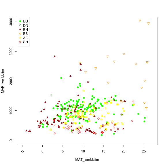
We may want to explore some of the patterns in the metadata before we jump into
specific locations. Let's look at Mean Annual Precipitation (MAP) and Mean Annual Temperature (MAT) across the different field site and classify those by the primary vegetation type ('primary_veg_type') for each site.
To do this we'd first want to remove the sites where there is not data and then
plot the data.
# #Some sites do not have data on Mean Annual Precipitation (MAP) and Mean Annual Temperature (MAT).
# removing the sites with unknown MAT and MAP values
phenos <- phenos[!((MAT_worldclim == -9999)|(MAP_worldclim == -9999))]
# Making a plot showing all sites by their vegetation type (represented as different symbols and colors) plotting across meteorology (MAT and MAP) space. Refer to table to identify vegetation type acronyms.
phenos[primary_veg_type=='DB', plot(MAT_worldclim, MAP_worldclim, pch = 19, col = 'green', xlim = c(-5, 27), ylim = c(0, 4000))]
#> NULL
phenos[primary_veg_type=='DN', points(MAT_worldclim, MAP_worldclim, pch = 1, col = 'darkgreen')]
#> NULL
phenos[primary_veg_type=='EN', points(MAT_worldclim, MAP_worldclim, pch = 17, col = 'brown')]
#> NULL
phenos[primary_veg_type=='EB', points(MAT_worldclim, MAP_worldclim, pch = 25, col = 'orange')]
#> NULL
phenos[primary_veg_type=='AG', points(MAT_worldclim, MAP_worldclim, pch = 12, col = 'yellow')]
#> NULL
phenos[primary_veg_type=='SH', points(MAT_worldclim, MAP_worldclim, pch = 23, col = 'red')]
#> NULL
legend('topleft', legend = c('DB','DN', 'EN','EB','AG', 'SH'),
pch = c(19, 1, 17, 25, 12, 23),
col = c('green', 'darkgreen', 'brown', 'orange', 'yellow', 'red' ))
Filtering using attributes
Alternatively, we may want to only include Phenocams with certain attributes in
our datasets. For example, we may be interested only in sites with a co-located
flux tower. For this, we'd want to filter for those with a flux tower using the
flux_sitenames attribute in the metadata.
# Create a data table only including the sites that have flux_data available and where the FLUX site name is specified
phenofluxsites <- phenos[flux_data==TRUE&!is.na(flux_sitenames)&flux_sitenames!='',
.(PhenoCam=site, Flux=flux_sitenames)] # return as table
#Specify to retain variables of Phenocam site and their flux tower name
phenofluxsites <- phenofluxsites[Flux!='']
# view the first few rows of the data table
head(phenofluxsites)
#> PhenoCam Flux
#> <char> <char>
#> 1: admixpasture NZ-ADw
#> 2: alercecosteroforest CL-ACF
#> 3: alligatorriver US-NC4
#> 4: amtsvenn No
#> 5: arkansaswhitaker US-RGW
#> 6: arsbrooks10 US-Br1: Brooks Field Site 10- Ames
We could further identify which of those Phenocams with a flux tower and in
deciduous broadleaf forests (primary_veg_type=='DB').
#list deciduous broadleaf sites with a flux tower
DB.flux <- phenos[flux_data==TRUE&primary_veg_type=='DB',
site] # return just the site names as a list
# see the first few rows
head(DB.flux)
#> [1] "alligatorriver" "bartlett" "bartlettir" "bbc1" "bbc2"
#> [6] "bbc3"
PhenoCam time series
PhenoCam time series are extracted time series data obtained from regions of interest (ROI's) for a given site.
Obtain ROIs
To download the phenological time series from the PhenoCam, we need to know the
site name, vegetation type and ROI ID. This information can be obtained from each
specific PhenoCam page on the
PhenoCam website
or by using the get_rois() function.
# Obtaining the list of all the available regions of interest (ROI's) on the PhenoCam server and producing a data table
rois <- get_rois()
# view the data variables in the data table
colnames(rois)
#> [1] "roi_name" "site" "lat" "lon"
#> [5] "roitype" "active" "show_link" "show_data_link"
#> [9] "sequence_number" "description" "first_date" "last_date"
#> [13] "site_years" "missing_data_pct" "roi_page" "roi_stats_file"
#> [17] "one_day_summary" "three_day_summary" "data_release"
# view first few regions of of interest (ROI) locations
head(rois$roi_name)
#> [1] "aafcottawacfiaf14n_AG_1000" "admixpasture_AG_1000" "adrycpasture_AG_1000"
#> [4] "alercecosteroforest_EN_1000" "alligatorriver_DB_1000" "almondifapa_AG_1000"
Download time series
The get_pheno_ts() function can download a time series and return the result
as a data.table.
Let's work with the
Duke Forest Hardwood Stand (dukehw) PhenoCam
and specifically the ROI
DB_1000
we can run the following code.
# list ROIs for dukehw
rois[site=='dukehw',]
#> roi_name site lat lon roitype active show_link show_data_link
#> <char> <char> <num> <num> <char> <lgcl> <lgcl> <lgcl>
#> 1: dukehw_DB_1000 dukehw 35.97358 -79.10037 DB TRUE TRUE TRUE
#> sequence_number description first_date last_date site_years
#> <num> <char> <char> <char> <char>
#> 1: 1000 canopy level DB forest at awesome Duke forest 2013-06-01 2024-12-30 10.7
#> missing_data_pct roi_page
#> <char> <char>
#> 1: 8.0 https://phenocam.nau.edu/webcam/roi/dukehw/DB_1000/
#> roi_stats_file
#> <char>
#> 1: https://phenocam.nau.edu/data/archive/dukehw/ROI/dukehw_DB_1000_roistats.csv
#> one_day_summary
#> <char>
#> 1: https://phenocam.nau.edu/data/archive/dukehw/ROI/dukehw_DB_1000_1day.csv
#> three_day_summary data_release
#> <char> <lgcl>
#> 1: https://phenocam.nau.edu/data/archive/dukehw/ROI/dukehw_DB_1000_3day.csv NA
# Obtain the decidous broadleaf, ROI ID 1000 data from the dukehw phenocam
dukehw_DB_1000 <- get_pheno_ts(site = 'dukehw', vegType = 'DB', roiID = 1000, type = '3day')
# Produces a list of the dukehw data variables
str(dukehw_DB_1000)
#> Classes 'data.table' and 'data.frame': 1414 obs. of 35 variables:
#> $ date : chr "2013-06-01" "2013-06-04" "2013-06-07" "2013-06-10" ...
#> $ year : int 2013 2013 2013 2013 2013 2013 2013 2013 2013 2013 ...
#> $ doy : int 152 155 158 161 164 167 170 173 176 179 ...
#> $ image_count : int 57 76 77 77 77 78 21 0 0 0 ...
#> $ midday_filename : chr "dukehw_2013_06_01_120111.jpg" "dukehw_2013_06_04_120119.jpg" "dukehw_2013_06_07_120112.jpg" "dukehw_2013_06_10_120108.jpg" ...
#> $ midday_r : num 91.3 76.4 60.6 76.5 88.9 ...
#> $ midday_g : num 97.9 85 73.2 82.2 95.7 ...
#> $ midday_b : num 47.4 33.6 35.6 37.1 51.4 ...
#> $ midday_gcc : num 0.414 0.436 0.432 0.42 0.406 ...
#> $ midday_rcc : num 0.386 0.392 0.358 0.391 0.377 ...
#> $ r_mean : num 87.6 79.9 72.7 80.9 83.8 ...
#> $ r_std : num 5.9 6 9.5 8.23 5.89 ...
#> $ g_mean : num 92.1 86.9 84 88 89.7 ...
#> $ g_std : num 6.34 5.26 7.71 7.77 6.47 ...
#> $ b_mean : num 46.1 38 39.6 43.1 46.7 ...
#> $ b_std : num 4.48 3.42 5.29 4.73 4.01 ...
#> $ gcc_mean : num 0.408 0.425 0.429 0.415 0.407 ...
#> $ gcc_std : num 0.00859 0.0089 0.01318 0.01243 0.01072 ...
#> $ gcc_50 : num 0.408 0.427 0.431 0.416 0.407 ...
#> $ gcc_75 : num 0.414 0.431 0.435 0.424 0.415 ...
#> $ gcc_90 : num 0.417 0.434 0.44 0.428 0.421 ...
#> $ rcc_mean : num 0.388 0.39 0.37 0.381 0.38 ...
#> $ rcc_std : num 0.01176 0.01032 0.01326 0.00881 0.00995 ...
#> $ rcc_50 : num 0.387 0.391 0.373 0.383 0.382 ...
#> $ rcc_75 : num 0.391 0.396 0.378 0.388 0.385 ...
#> $ rcc_90 : num 0.397 0.399 0.382 0.391 0.389 ...
#> $ max_solar_elev : num 76 76.3 76.6 76.8 76.9 ...
#> $ snow_flag : logi NA NA NA NA NA NA ...
#> $ outlierflag_gcc_mean: logi NA NA NA NA NA NA ...
#> $ outlierflag_gcc_50 : logi NA NA NA NA NA NA ...
#> $ outlierflag_gcc_75 : logi NA NA NA NA NA NA ...
#> $ outlierflag_gcc_90 : logi NA NA NA NA NA NA ...
#> $ YEAR : int 2013 2013 2013 2013 2013 2013 2013 2013 2013 2013 ...
#> $ DOY : int 152 155 158 161 164 167 170 173 176 179 ...
#> $ YYYYMMDD : chr "2013-06-01" "2013-06-04" "2013-06-07" "2013-06-10" ...
#> - attr(*, ".internal.selfref")=<externalptr>
We now have a variety of data related to this ROI from the Hardwood Stand at Duke
Forest.
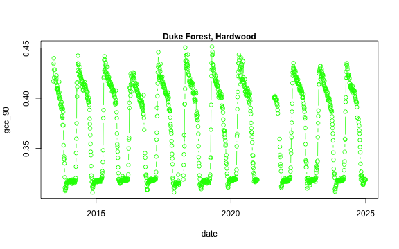
Green Chromatic Coordinate (GCC) is a measure of "greenness" of an area and is
widely used in Phenocam images as an indicator of the green pigment in vegetation.
Let's use this measure to look at changes in GCC over time at this site. Looking
back at the available data, we have several options for GCC. gcc90 is the 90th
quantile of GCC in the pixels across the ROI (for more details,
PhenoCam v1 description).
We'll use this as it tracks the upper greenness values while not including many
outliners.
Before we can plot gcc-90 we do need to fix our dates and convert them from
Factors to Date to correctly plot.
# Convert date variable into date format
dukehw_DB_1000[,date:=as.Date(date)]
# plot gcc_90
dukehw_DB_1000[,plot(date, gcc_90, col = 'green', type = 'b')]
#> NULL
mtext('Duke Forest, Hardwood', font = 2)
Download midday images
While PhenoCam sites may have many images in a given day, many simple analyses
can use just the midday image when the sun is most directly overhead the canopy.
Therefore, extracting a list of midday images (only one image a day) can be useful.
# obtaining midday_images for dukehw
duke_middays <- get_midday_list('dukehw')
# see the first few rows
head(duke_middays)
#> [1] "http://phenocam.nau.edu/data/archive/dukehw/2013/05/dukehw_2013_05_31_150331.jpg"
#> [2] "http://phenocam.nau.edu/data/archive/dukehw/2013/06/dukehw_2013_06_01_120111.jpg"
#> [3] "http://phenocam.nau.edu/data/archive/dukehw/2013/06/dukehw_2013_06_02_120109.jpg"
#> [4] "http://phenocam.nau.edu/data/archive/dukehw/2013/06/dukehw_2013_06_03_120110.jpg"
#> [5] "http://phenocam.nau.edu/data/archive/dukehw/2013/06/dukehw_2013_06_04_120119.jpg"
#> [6] "http://phenocam.nau.edu/data/archive/dukehw/2013/06/dukehw_2013_06_05_120110.jpg"
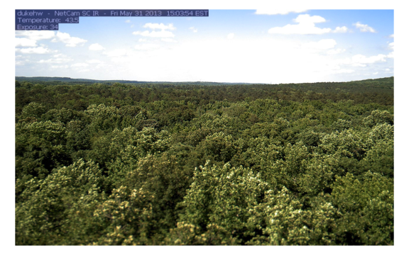
Now we have a list of all the midday images from this Phenocam. Let's download
them and plot
# download a file
destfile <- tempfile(fileext = '.jpg')
# download only the first available file
# modify the `[1]` to download other images
download.file(duke_middays[1], destfile = destfile, mode = 'wb')
# plot the image
img <- try(readJPEG(destfile))
if(class(img)!='try-error'){
par(mar= c(0,0,0,0))
plot(0:1,0:1, type='n', axes= FALSE, xlab= '', ylab = '')
rasterImage(img, 0, 0, 1, 1)
}
Download midday images for a given time range
Now we can access all the midday images and download them one at a time. However,
we frequently want all the images within a specific time range of interest. We'll
learn how to do that next.
# open a temporary directory
tmp_dir <- tempdir()
# download a subset. Example dukehw 2017
download_midday_images(site = 'dukehw', # which site
y = 2017, # which year(s)
months = 1:12, # which month(s)
days = 15, # which days on month(s)
download_dir = tmp_dir) # where on your computer
# list of downloaded files
duke_middays_path <- dir(tmp_dir, pattern = 'dukehw*', full.names = TRUE)
head(duke_middays_path)
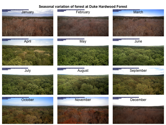
We can demonstrate the seasonality of Duke forest observed from the camera. (Note
this code may take a while to run through the loop).
n <- length(duke_middays_path)
par(mar= c(0,0,0,0), mfrow=c(4,3), oma=c(0,0,3,0))
for(i in 1:n){
img <- readJPEG(duke_middays_path[i])
plot(0:1,0:1, type='n', axes= FALSE, xlab= '', ylab = '')
rasterImage(img, 0, 0, 1, 1)
mtext(month.name[i], line = -2)
}
mtext('Seasonal variation of forest at Duke Hardwood Forest', font = 2, outer = TRUE)
The goal of this section was to show how to download a limited number of midday images from the PhenoCam server. However, more extensive datasets should be downloaded from the PhenoCam .
In this tutorial, we'll learn how to use an interactive open-source toolkit, the
xROI
that facilitates the process of time series extraction and improves the quality
of the final data. The xROI package provides a responsive environment for
scientists to interactively:
a) delineate regions of interest (ROIs),
b) handle field of view (FOV) shifts, and
c) extract and export time series data characterizing color-based metrics.
Using the xROI R package, the user can detect FOV shifts with minimal difficulty.
The software gives user the opportunity to re-adjust mask files or redraw new
ones every time an FOV shift occurs.
xROI Design
The R language and Shiny package were used as the main development tool for xROI,
while Markdown, HTML, CSS and JavaScript languages were used to improve the
interactivity. While Shiny apps are primarily used for web-based applications to
be used online, the package authors used Shiny for its graphical user interface
capabilities. In other words, both the User Interface (UI) and server modules are run
locally from the same machine and hence no internet connection is required (after
installation). The xROI's UI element presents a side-panel for data entry and
three main tab-pages, each responsible for a specific task. The server-side
element consists of R and bash scripts. Image processing and geospatial features
were performed using the Geospatial Data Abstraction Library (GDAL) and the
rgdal and raster R packages.
Install xROI
The latest release of xROI can be directly downloaded and installed from the development GitHub repository.
# install devtools first
utils::install.packages('devtools', repos = "http://cran.us.r-project.org" )
# use devtools to install from GitHub
devtools::install_github("bnasr/xROI")
xROI depends on many R packages including: raster, rgdal, sp, jpeg,
tiff, shiny, shinyjs, shinyBS, shinyAce, shinyTime, shinyFiles,
shinydashboard, shinythemes, colourpicker, rjson, stringr, data.table,
lubridate, plotly, moments, and RCurl. All the required libraries and
packages will be automatically installed with installation of xROI. The package
offers a fully interactive high-level interface as well as a set of low-level
functions for ROI processing.
Launch xROI
A comprehensive user manual for low-level image processing using xROI is available from
GitHub xROI.
While the user manual includes a set of examples for each function; here we
will learn to use the graphical interactive mode.
Calling the Launch() function, as we'll do below, opens up the interactive
mode in your operating system’s default web browser. The landing page offers an
example dataset to explore different modules or upload a new dataset of images.
You can launch the interactive mode can be launched from an interactive R environment.
# load xROI
library(xROI)
# launch xROI
Launch()
Or from the command line (e.g. bash in Linux, Terminal in macOS and Command
Prompt in Windows machines) where an R engine is already installed.
Rscript -e “xROI::Launch(Interactive = TRUE)”
End xROI
When you are done with the xROI interface you can close the tab in your browser
and end the session in R by using one of the following options
In RStudio: Press the key on your keyboard.
In R Terminal: Press <Ctrl + C> on your keyboard.
Use xROI
To get some hands-on experience with xROI, we can analyze images from the
dukehw
of the PhenoCam network.
First,save and extract (unzip) the file on your computer.
Second, open the data set in xROI by setting the file path to your data
# launch data in ROI
# first edit the path below to the dowloaded directory you just extracted
xROI::Launch('/path/to/extracted/directory')
# alternatively, you can run without specifying a path and use the interface to browse
Now, draw an ROI and the metadata.
Then, save the metadata and explore its content.
Now we can explore if there is any FOV shift in the dataset using the CLI processer tab.
Finally, we can go to the Time series extraction tab. Extract the time-series. Save the output and explore the dataset in R.
Challenge: Use xROI
Let's use xROI on a little more challenging site with field of view shifts.
Before we start the image processing steps, let's read in and plot an image. This
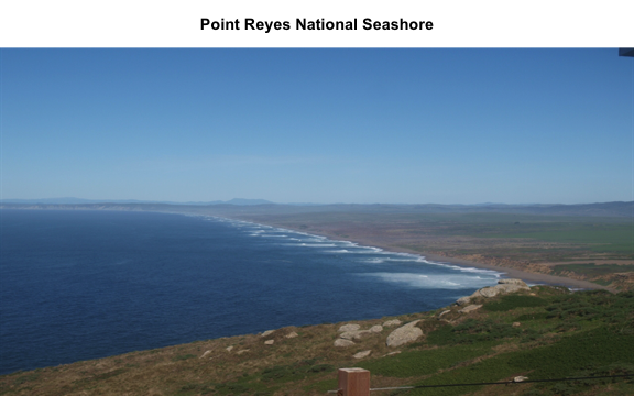
image is an example image that comes with the hazer package.
# read the path to the example image
jpeg_file <- system.file(package = 'hazer', 'pointreyes.jpg')
# read the image as an array
rgb_array <- jpeg::readJPEG(jpeg_file)
# plot the RGB array on the active device panel
# first set the margin in this order:(bottom, left, top, right)
par(mar=c(0,0,3,0))
plotRGBArray(rgb_array, bty = 'n', main = 'Point Reyes National Seashore')
When we work with images, all data we work with is generally on the scale of each
individual pixel in the image. Therefore, for large images we will be working with
large matrices that hold the value for each pixel. Keep this in mind before opening
some of the matrices we'll be creating this tutorial as it can take a while for
them to load.
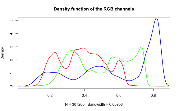
Histogram of RGB channels
A histogram of the colors can be useful to understanding what our image is made
up of. Using the density() function from the base stats package, we can extract
density distribution of each color channel.
# color channels can be extracted from the matrix
red_vector <- rgb_array[,,1]
green_vector <- rgb_array[,,2]
blue_vector <- rgb_array[,,3]
# plotting
par(mar=c(5,4,4,2))
plot(density(red_vector), col = 'red', lwd = 2,
main = 'Density function of the RGB channels', ylim = c(0,5))
lines(density(green_vector), col = 'green', lwd = 2)
lines(density(blue_vector), col = 'blue', lwd = 2)
In hazer we can also extract three basic elements of an RGB image :
Brightness
Darkness
Contrast
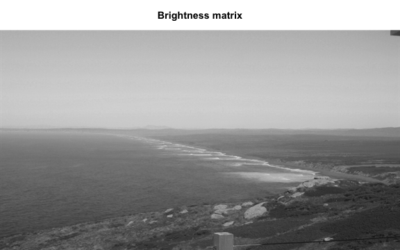
Brightness
The brightness matrix comes from the maximum value of the R, G, or B channel. We
can extract and show the brightness matrix using the getBrightness() function.
# extracting the brightness matrix
brightness_mat <- getBrightness(rgb_array)
# unlike the RGB array which has 3 dimensions, the brightness matrix has only two
# dimensions and can be shown as a grayscale image,
# we can do this using the same plotRGBArray function
par(mar=c(0,0,3,0))
plotRGBArray(brightness_mat, bty = 'n', main = 'Brightness matrix')
Here the grayscale is used to show the value of each pixel's maximum brightness
of the R, G or B color channel.
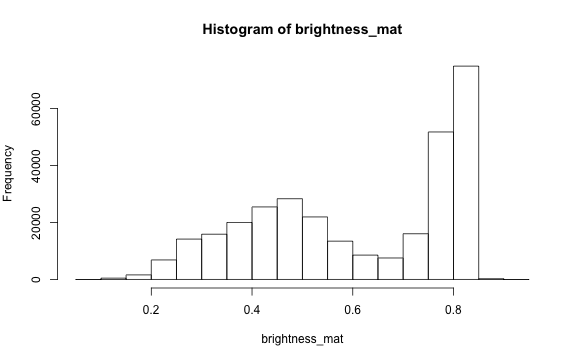
To extract a single brightness value for the image, depending on our needs we can
perform some statistics or we can just use the mean of this matrix.
Why are we getting so many images up in the high range of the brightness? Where
does this correlate to on the RGB image?
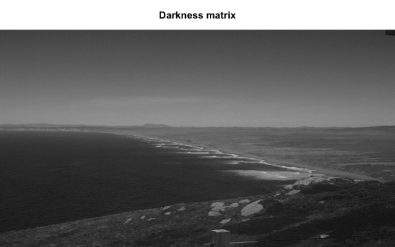
Darkness
Darkness is determined by the minimum of the R, G or B color channel.
Similarly, we can extract and show the darkness matrix using the getDarkness() function.
# extracting the darkness matrix
darkness_mat <- getDarkness(rgb_array)
# the darkness matrix has also two dimensions and can be shown as a grayscale image
par(mar=c(0,0,3,0))
plotRGBArray(darkness_mat, bty = 'n', main = 'Darkness matrix')
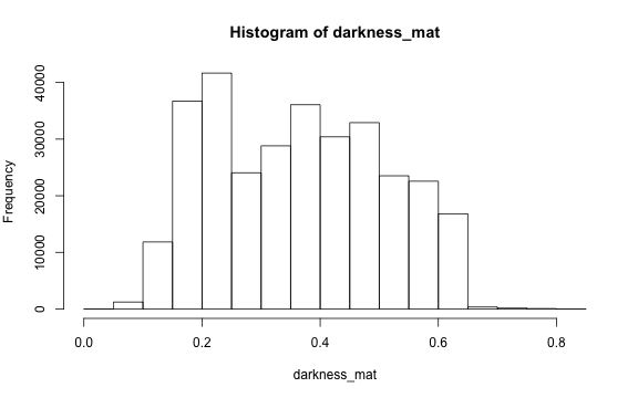
# main quantiles
quantile(darkness_mat)
#> 0% 25% 50% 75% 100%
#> 0.03529412 0.23137255 0.36470588 0.47843137 0.83529412
# histogram
par(mar=c(5,4,4,2))
hist(darkness_mat)
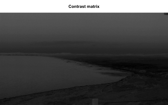
Contrast
The contrast of an image is the difference between the darkness and brightness
of the image. The contrast matrix is calculated by difference between the
darkness and brightness matrices.
The contrast of the image can quickly be extracted using the getContrast() function.
# extracting the contrast matrix
contrast_mat <- getContrast(rgb_array)
# the contrast matrix has also 2D and can be shown as a grayscale image
par(mar=c(0,0,3,0))
plotRGBArray(contrast_mat, bty = 'n', main = 'Contrast matrix')
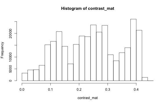
# main quantiles
quantile(contrast_mat)
#> 0% 25% 50% 75% 100%
#> 0.0000000 0.1450980 0.2470588 0.3333333 0.4509804
# histogram
par(mar=c(5,4,4,2))
hist(contrast_mat)
Image fogginess & haziness
Haziness of an image can be estimated using the getHazeFactor() function. This
function is based on the method described in
Mao et al. (2014).
The technique was originally developed to for "detecting foggy images and
estimating the haze degree factor" for a wide range of outdoor conditions.
The function returns a vector of two numeric values:
haze as the haze degree and
A0 as the global atmospheric light, as it is explained in the original paper.
The PhenoCam standards classify any image with the haze degree greater
than 0.4 as a significantly foggy image.
Download and extract the zip file to be used as input data for the following step.
# to download via R
dir.create('data')
#> Warning in dir.create("data"): 'data' already exists
destfile = 'data/pointreyes.zip'
download.file(destfile = destfile, mode = 'wb', url = 'http://bit.ly/2F8w2Ia')
unzip(destfile, exdir = 'data')
# set up the input image directory
#pointreyes_dir <- '/path/to/image/directory/'
pointreyes_dir <- 'data/pointreyes/'
# get a list of all .jpg files in the directory
pointreyes_images <- dir(path = pointreyes_dir,
pattern = '*.jpg',
ignore.case = TRUE,
full.names = TRUE)
Now we can use a for loop to process all of the images to get the haze and A0
values.
(Note, this loop may take a while to process.)
# number of images
n <- length(pointreyes_images)
# create an empty matrix to fill with haze and A0 values
haze_mat <- data.table()
# the process takes a bit, a progress bar lets us know it is working.
pb <- txtProgressBar(0, n, style = 3)
#>
Now we can save all the foggy images to a new folder that will retain the
foggy images but keep them separate from the non-foggy ones that we want to
analyze.
# identify directory to move the foggy images to
foggy_dir <- paste0(pointreyes_dir, 'foggy')
clear_dir <- paste0(pointreyes_dir, 'clear')
# if a new directory, create new directory at this file path
dir.create(foggy_dir, showWarnings = FALSE)
dir.create(clear_dir, showWarnings = FALSE)
# copy the files to the new directories
file.copy(haze_mat[foggy==TRUE,file], to = foggy_dir)
#> [1] FALSE FALSE FALSE FALSE FALSE FALSE FALSE FALSE FALSE FALSE FALSE FALSE FALSE FALSE
#> [15] FALSE FALSE FALSE FALSE FALSE FALSE FALSE FALSE FALSE FALSE FALSE FALSE FALSE FALSE
#> [29] FALSE FALSE
file.copy(haze_mat[foggy==FALSE,file], to = clear_dir)
#> [1] FALSE FALSE FALSE FALSE FALSE FALSE FALSE FALSE FALSE FALSE FALSE FALSE FALSE FALSE
#> [15] FALSE FALSE FALSE FALSE FALSE FALSE FALSE FALSE FALSE FALSE FALSE FALSE FALSE FALSE
#> [29] FALSE FALSE FALSE FALSE FALSE FALSE FALSE FALSE FALSE FALSE FALSE FALSE FALSE
Now that we have our images separated, we can get the full list of haze
values only for those images that are not classified as "foggy".
# this is an alternative approach instead of a for loop
# loading all the images as a list of arrays
pointreyes_clear_images <- dir(path = clear_dir,
pattern = '*.jpg',
ignore.case = TRUE,
full.names = TRUE)
img_list <- lapply(pointreyes_clear_images, FUN = jpeg::readJPEG)
# getting the haze value for the list
# patience - this takes a bit of time
haze_list <- t(sapply(img_list, FUN = getHazeFactor))
# view first few entries
head(haze_list)
#> haze A0
#> [1,] 0.224981 0.6970257
#> [2,] 0.2339372 0.6826148
#> [3,] 0.231294 0.7009978
#> [4,] 0.2297961 0.6813884
#> [5,] 0.2152078 0.6949932
#> [6,] 0.345584 0.6789334
We can then use these values for further analyses and data correction.
This tutorial covers downloading NEON data, using the Data Portal and
either the neonUtilities R package or the neonutilities Python package,
as well as basic instruction in beginning to explore and work with the
downloaded data, including guidance in navigating data documentation. We
will explore data of 3 different types, and make a simple figure from
each.
NEON data
There are 3 basic categories of NEON data:
Remote sensing (AOP) - Data collected by the airborne observation
platform, e.g. LIDAR, surface reflectance
Observational (OS) - Data collected by a human in the field, or in
an analytical laboratory, e.g. beetle identification, foliar
isotopes
Instrumentation (IS) - Data collected by an automated, streaming
sensor, e.g. net radiation, soil carbon dioxide. This category also
includes the surface-atmosphere exchange (SAE) data, which are processed
and structured in a unique way, distinct from other instrumentation data
(see the introductory
eddy
flux data tutorial for details).
This lesson covers all three types of data. The download procedures
are similar for all types, but data navigation differs significantly by
type.
Objectives
After completing this activity, you will be able to:
Download NEON data using the neonUtilities package.
Understand downloaded data sets and load them into R or Python for
analyses.
Things You’ll Need To Complete This Tutorial
You can follow either the R or Python code throughout this tutorial.
* For R users, we recommend using R version 4+ and RStudio. * For Python
users, we recommend using Python 3.9+.
Set up: Install Packages
Packages only need to be installed once, you can skip this step after
the first time:
R
neonUtilities: Basic functions for accessing NEON
data
neonOS: Functions for common data wrangling needs
for NEON observational data.
terra: Spatial data package; needed for working
with remote sensing data.
import neonutilities as nu
import os
import rasterio
import pandas as pd
import matplotlib.pyplot as plt
Getting started: Download data from the Portal
Go to the NEON
Data Portal and download some data! To follow the tutorial exactly,
download Photosynthetically active radiation (PAR) (DP1.00024.001) data
from September-November 2019 at Wind River Experimental Forest (WREF).
The downloaded file should be a zip file named NEON_par.zip.
If you prefer to explore a different data product, you can still
follow this tutorial. But it will be easier to understand the steps in
the tutorial, particularly the data navigation, if you choose a sensor
data product for this section.
Once you’ve downloaded a zip file of data from the portal, switch
over to R or Python to proceed with coding.
Stack the downloaded data files: stackByTable()
The stackByTable() (or stack_by_table())
function will unzip and join the files in the downloaded zip file.
R
# Modify the file path to match the path to your zip file
stackByTable("~/Downloads/NEON_par.zip")
Python
# Modify the file path to match the path to your zip file
nu.stack_by_table(os.path.expanduser("~/Downloads/NEON_par.zip"))
In the directory where the zipped file was saved, you should now have
an unzipped folder of the same name. When you open this you will see a
new folder called stackedFiles, which should contain at
least seven files: PARPAR_30min.csv,
PARPAR_1min.csv, sensor_positions.csv,
variables_00024.csv, readme_00024.txt,
issueLog_00024.csv, and
citation_00024_RELEASE-202X.txt.
Navigate data downloads: IS
Let’s start with a brief description of each file. This set of files
is typical of a NEON IS data product.
PARPAR_30min.csv: PAR data at 30-minute averaging
intervals
PARPAR_1min.csv: PAR data at 1-minute averaging
intervals
sensor_positions.csv: The physical location of each
sensor collecting PAR measurements. There is a PAR sensor at each level
of the WREF tower, and this table lets you connect the tower level index
to the height of the sensor in meters.
variables_00024.csv: Definitions and units for each
data field in the PARPAR_#min tables.
readme_00024.txt: Basic information about the PAR
data product.
issueLog_00024.csv: A record of known issues
associated with PAR data.
citation_00024_RELEASE-202X.txt: The citation to
use when you publish a paper using these data, in BibTeX format.
We’ll explore the 30-minute data. To read the file, use the function
readTableNEON() or read_table_neon(), which
uses the variables file to assign data types to each column of data:
par30 = nu.read_table_neon(
data_file=os.path.expanduser(
"~/Downloads/NEON_par/stackedFiles/PARPAR_30min.csv"),
var_file=os.path.expanduser(
"~/Downloads/NEON_par/stackedFiles/variables_00024.csv"))
# Open the par30 table in the table viewer of your choice
The first four columns are added by stackByTable() when
it merges files across sites, months, and tower heights. The column
publicationDate is the date-time stamp indicating when the
data were published, and the release column indicates which
NEON data release the data belong to. For more information about NEON
data releases, see the
Data
Product Revisions and Releases page.
Information about each data column can be found in the variables
file, where you can see definitions and units for each column of
data.
Plot PAR data
Now that we know what we’re looking at, let’s plot PAR from the top
tower level. We’ll use the mean PAR from each averaging interval, and we
can see from the sensor positions file that the vertical index 080
corresponds to the highest tower level. To explore the sensor positions
data in more depth, see the
spatial
data tutorial.
We can see there is a lot of light attenuation through the
canopy.
Download files and load directly to R:
loadByProduct()
At the start of this tutorial, we downloaded data from the NEON data
portal. NEON also provides an API, and the neonUtilities
packages provide methods for downloading programmatically.
The steps we carried out above - downloading from the portal,
stacking the downloaded files, and reading in to R or Python - can all
be carried out in one step by the neonUtilities function
loadByProduct().
To get the same PAR data we worked with above, we would run this line
of code using loadByProduct():
The object returned by loadByProduct() in R is a named
list, and the object returned by load_by_product() in
Python is a dictionary. The objects contained in the list or dictionary
are the same set of tables we ended with after stacking the data from
the portal above. You can see this by checking the names of the tables
in parlist:
Now let’s walk through the details of the inputs and options in
loadByProduct().
This function downloads data from the NEON API, merges the
site-by-month files, and loads the resulting data tables into the
programming environment, assigning each data type to the appropriate
class. This is a popular choice for NEON data users because it ensures
you’re always working with the latest data, and it ends with
ready-to-use tables. However, if you use it in a workflow you run
repeatedly, keep in mind it will re-download the data every time. See
below for suggestions on saving the data locally to save time and
compute resources.
loadByProduct() works on most observational (OS) and
sensor (IS) data, but not on surface-atmosphere exchange (SAE) data and remote sensing (AOP) data. For functions that download AOP data, see the final
section in this tutorial. For functions that work with SAE data, see the
NEON
eddy flux data tutorial.
The inputs to loadByProduct() control which data to
download and how to manage the processing. The list below shows the R syntax; in Python,
the inputs are the same but all lowercase (e.g. `dpid` instead of `dpID`)
and `.` is replaced by `_`.
dpID: the data product ID, e.g. DP1.00002.001
site: defaults to “all”, meaning all sites with
available data; can be a vector of 4-letter NEON site codes, e.g.
c("HARV","CPER","ABBY") (or
["HARV","CPER","ABBY"] in Python)
startdate and enddate: defaults to NA,
meaning all dates with available data; or a date in the form YYYY-MM,
e.g. 2017-06. Since NEON data are provided in month packages, finer
scale querying is not available. Both start and end date are
inclusive.
package: either basic or expanded data package.
Expanded data packages generally include additional information about
data quality, such as chemical standards and quality flags. Not every
data product has an expanded package; if the expanded package is
requested but there isn’t one, the basic package will be
downloaded.
timeIndex: defaults to “all”, to download all data; or
the number of minutes in the averaging interval. Only applicable to IS
data.
release: Specify a NEON data release to download.
Defaults to the most recent release plus provisional data. See the
release
tutorial for more information.
include.provisional: T or F: should Provisional data be
included in the download? Defaults to F to return only Released data,
which are citable by a DOI and do not change over time. Provisional data
are subject to change.
check.size: T or F: should the function pause before
downloading data and warn you about the size of your download? Defaults
to T; if you are using this function within a script or batch process
you will want to set it to F.
token: Optional NEON API token for faster downloads.
See
this
tutorial for instructions on using a token.
progress: Set to F to turn off progress bars.
cloud.mode: Can be set to T if you are working in a
cloud environment; enables more efficient data transfer from NEON’s
cloud storage.
The dpID is the data product identifier of the data you
want to download. The DPID can be found on the
Explore Data Products page. It will be in the form DP#.#####.###
Download observational data
To explore observational data, we’ll download aquatic plant chemistry
data (DP1.20063.001) from three lake sites: Prairie Lake (PRLA), Suggs
Lake (SUGG), and Toolik Lake (TOOK).
As we saw above, the object returned by loadByProduct()
is a named list of data frames. Let’s check out what’s the same and
what’s different from the IS data tables.
As with the sensor data, we have some data tables and some metadata
tables. Most of the metadata files are the same as the sensor data:
readme, variables,
issueLog, and citation. These files
contain the same type of metadata here that they did in the IS data
product. Let’s look at the other files:
apl_clipHarvest: Data from the clip harvest
collection of aquatic plants
apl_biomass: Biomass data from the collected
plants
apl_plantExternalLabDataPerSample: Chemistry data
from the collected plants
apl_plantExternalLabQA: Quality assurance data from
the chemistry analyses
asi_externalLabPOMSummaryData: Quality metrics from
the chemistry lab
validation_20063: For observational data, a major
method for ensuring data quality is to control data entry. This file
contains information about the data ingest rules applied to each input
data field.
categoricalCodes_20063: Definitions of each value
for categorical data, such as growth form and sample condition
You can work with these tables from the named list object, but many
people find it easier to extract each table from the list and work with
it as an independent object. To do this, use the list2env()
function in R or globals().update() in Python:
R
list2env(apchem, .GlobalEnv)
## <environment: R_GlobalEnv>
Python
globals().update(apchem)
Save data locally
Keep in mind that using loadByProduct() will re-download
the data every time you run your code. In some cases this may be
desirable, but it can be a waste of time and compute resources. To come
back to these data without re-downloading, you’ll want to save the
tables locally. The most efficient option is to save the named list in
total - this will also preserve the data types.
R
saveRDS(apchem,
"~/Downloads/aqu_plant_chem.rds")
Python
# There are a variety of ways to do this in Python; NEON
# doesn't currently have a specific recommendation. If
# you don't have a data-saving workflow you already use,
# we suggest you check out the pickle module.
Then you can re-load the object to a programming environment any
time.
Other options for saving data locally:
Similar to the workflow we started this tutorial with, but using
neonUtilities to download instead of the Portal: Use
zipsByProduct() and stackByTable() instead of
loadByProduct(). With this option, use the function
readTableNEON() to read the files, to get the same column
type assignment that loadByProduct() carries out. Details
can be found in our
neonUtilities
tutorial.
Try out the community-developed neonstore package,
which is designed for maintaining a local store of the NEON data you
use. The neonUtilities function
stackFromStore() works with files downloaded by
neonstore. See the
neonstore
tutorial for more information.
Now let’s explore the aquatic plant data. OS data products are simple
in that the data are generally tabular, and data volumes are lower than the other NEON data types, but they are complex in that almost all consist
of multiple tables containing information collected at different times
in different ways. For example, samples collected in the field may be
shipped to a laboratory for analysis. Data associated with the field
collection will appear in one data table, and the analytical results
will appear in another. Complexity in working with OS data usually
involves bringing data together from multiple measurements or scales of
analysis.
As with the IS data, the variables file can tell you more about the
data tables.
OS data products each come with a Data Product User Guide, which can
be downloaded with the data, or accessed from the document library on
the Data Portal, or the
Product
Details page for the data product. The User Guide is designed to
give a basic introduction to the data product, including a brief summary
of the protocol and descriptions of data format and structure.
Explore isotope data
To get started with the aquatic plant chemistry data, let’s take a
look at carbon isotope ratios in plants across the three sites we
downloaded. The chemical analytes are reported in the
apl_plantExternalLabDataPerSample table, and the table is
in long format, with one record per sample per analyte, so we’ll subset
to only the carbon isotope analyte:
apl13C = apl_plantExternalLabDataPerSample[
apl_plantExternalLabDataPerSample.analyte=="d13C"]
grouped = apl13C.groupby("siteID")["analyteConcentration"]
fig, ax = plt.subplots()
ax.boxplot(x=[group.values for name, group in grouped],
tick_labels=grouped.groups.keys())
plt.show()
We see plants at Suggs and Toolik are quite low in 13C, with more
spread at Toolik than Suggs, and plants at Prairie Lake are relatively
enriched. Clearly the next question is what species these data
represent. But taxonomic data aren’t present in the
apl_plantExternalLabDataPerSample table, they’re in the
apl_biomass table. We’ll need to join the two tables to get
chemistry by taxon.
Every NEON data product has a Quick Start Guide (QSG), and for OS
products it includes a section describing how to join the tables in the
data product. Since it’s a pdf file, loadByProduct()
doesn’t bring it in, but you can view the Aquatic plant chemistry QSG on
the
Product
Details page. In R, the neonOS package uses the information
from the QSGs to provide an automated table-joining function,
joinTableNEON().
And now we can see most of the sampled plants have carbon isotope
ratios around -30, with just a few species accounting for most of the
more enriched samples.
Download remote sensing data: byFileAOP() and
byTileAOP()
Remote sensing data files are very large, so downloading them can
take a long time. byFileAOP() and byTileAOP()
enable easier programmatic downloads, but be aware it can take a very
long time to download large amounts of data.
Input options for the AOP functions are:
dpID: the data product ID, e.g. DP1.00002.001
site: the 4-letter code of a single site,
e.g. HARV
year: the 4-digit year to download
savepath: the file path you want to download to;
defaults to the working directory
check.size: T or F: should the function pause before
downloading data and warn you about the size of your download? Defaults
to T; if you are using this function within a script or batch process
you will want to set it to F.
easting: byTileAOP() only. Vector of
easting UTM coordinates whose corresponding tiles you want to
download
northing: byTileAOP() only. Vector of
northing UTM coordinates whose corresponding tiles you want to
download
buffer: byTileAOP() only. Size in meters
of buffer to include around coordinates when deciding which tiles to
download
token: Optional NEON API token for faster
downloads.
chunk_size: Only in Python. Set the chunk size of
chunked downloads, can improve efficiency in some cases. Defaults to 1
MB.
Here, we’ll download one tile of Ecosystem structure (Canopy Height
Model) (DP3.30015.001) from WREF in 2017.
In the directory indicated in savepath, you should now
have a folder named DP3.30015.001 with several nested
subfolders, leading to a tif file of a canopy height model tile.
Navigate data downloads: AOP
To work with AOP data, the best bet in R is the terra
package. It has functionality for most analyses you might want to do. In
Python, we’ll use the rasterio package here; explore NEON remote sensing
tutorials for more guidance.
Now we can see canopy height across the downloaded tile; the tallest
trees are over 60 meters, not surprising in the Pacific Northwest. There
is a clearing or clear cut in the lower right quadrant.
Next steps
Now that you’ve learned the basics of downloading and understanding
NEON data, where should you go to learn more? There are many more NEON
tutorials to explore, including how to align remote sensing and
ground-based measurements, a deep dive into the data quality flagging in
the sensor data products, and much more. For a recommended suite of
tutorials for new users, check out the
Getting
Started with NEON Data tutorial series.
In this tutorial, we will use the Spectral Python (SPy) package to run a KMeans unsupervised classification algorithm and then we will run Principal Component Analysis to reduce data dimensionality.
Objectives
After completing this tutorial, you will be able to:
Run kmeans unsupervised classification on AOP hyperspectral data
Reduce data dimensionality using Principal Component Analysis (PCA)
Install Python Packages
To run this notebook, the following Python packages need to be installed. You can install required packages from the command line (prior to opening your notebook), e.g. pip install gdal h5py neonutilities scikit-learn spectral requests. If already in a Jupyter Notebook, run the same command in a Code cell, but start with !pip install.
gdal
h5py
neonutilities
scikit-image
spectral
requests
For visualization (optional)
In order to make use of the interactive graphics capabilities of spectralpython, such as N-Dimensional Feature Display, you will need the additional packages below. These are not required to complete this lesson.
The data required for this lesson will be downloaded in the beginning of the tutorial using the Python neonutilities package.
In this tutorial, we will use the Spectral Python (SPy) package to run KMeans unsupervised classification algorithm as well as Principal Component Analysis (PCA).
To learn more about the Spectral Python packages read:
KMeans is an iterative clustering algorithm used to classify unsupervised data (eg. data without a training set) into a specified number of groups. The algorithm begins with an initial set of randomly determined cluster centers. Each pixel in the image is then assigned to the nearest cluster center (using distance in N-space as the distance metric) and each cluster center is then re-computed as the centroid of all pixels assigned to the cluster. This process repeats until a desired stopping criterion is reached (e.g. max number of iterations).
To visualize how the algorithm works, it's easier look at a 2D data set. In the example below, watch how the cluster centers shift with progressive iterations,
Principal Component Analysis (PCA) - Dimensionality Reduction
Many of the bands within hyperspectral images are often strongly correlated. The principal components transformation represents a linear transformation of the original image bands to a set of new, uncorrelated features. These new features correspond to the eigenvectors of the image covariance matrix, where the associated eigenvalue represents the variance in the direction of the eigenvector. A very large percentage of the image variance can be captured in a relatively small number of principal components (compared to the original number of bands).
For this example, we will download a bidirectional surface reflectance data cube at the SERC site, collected in 2022.
nu.by_tile_aop(dpid='DP3.30006.002',
site='SERC',
year='2022',
easting=368005,
northing=4306005,
include_provisional=True,
#token=your_token_here
savepath=os.path.join(data_dir)) # save to the home directory under a 'data' subfolder
Provisional data are included. To exclude provisional data, use input parameter include_provisional=False.
Continuing will download 2 files totaling approximately 692.0 MB. Do you want to proceed? (y/n) y
Let's see what data were downloaded.
# iterating over directory and subdirectory to get desired result
for root, dirs, files in os.walk(data_dir):
for name in files:
if name.endswith('.h5'):
print(os.path.join(root, name)) # printing file name
# function to download data stored on the internet in a public url to a local file
def download_url(url,download_dir):
if not os.path.isdir(download_dir):
os.makedirs(download_dir)
filename = url.split('/')[-1]
r = requests.get(url, allow_redirects=True)
file_object = open(os.path.join(download_dir,filename),'wb')
file_object.write(r.content)
module_url = "https://raw.githubusercontent.com/NEONScience/NEON-Data-Skills/main/tutorials/Python/AOP/aop_python_modules/neon_aop_hyperspectral.py"
download_url(module_url,'../python_modules')
# os.listdir('../python_modules') #optionally show the contents of this directory to confirm the file downloaded
sys.path.insert(0, '../python_modules')
# import the neon_aop_hyperspectral module, the semicolon supresses an empty plot from displaying
import neon_aop_hyperspectral as neon_hs;
# read in the reflectance data using the aop_h5refl2array function, this may also take a bit of time
start_time = time()
refl, refl_metadata, wavelengths = neon_hs.aop_h5refl2array(h5_tile,'Reflectance')
print("--- It took %s seconds to read in the data ---" % round((time() - start_time),0))
Reading in C:\Users\bhass\data\DP3.30006.002\neon-aop-provisional-products\2022\FullSite\D02\2022_SERC_6\L3\Spectrometer\Reflectance\NEON_D02_SERC_DP3_368000_4306000_bidirectional_reflectance.h5
--- It took 27.0 seconds to read in the data ---
The next few cells show how you can look at the contents, values, and dimensions of the refl_metadata, wavelengths, and refl variables, respectively.
print('First and last 5 center wavelengths, in nm:')
print(wavelengths[:5])
print(wavelengths[-5:])
First and last 5 center wavelengths, in nm:
[383.884003 388.891693 393.899506 398.907196 403.915009]
[2492.149414 2497.157227 2502.165039 2507.172607 2512.18042 ]
refl.shape
(1000, 1000, 426)
Next let's define a function to clean and subset the data.
def clean_neon_refl_data(data, metadata, wavelengths, subset_factor=1):
"""Clean h5 reflectance data and metadata
1. set data ignore value (-9999) to NaN
2. apply reflectance scale factor (10000)
3. remove bad bands (water vapor band windows + last 10 bands):
Band_Window_1_Nanometers = 1340, 1445
Band_Window_2_Nanometers = 1790, 1955
4. if subset_factor, subset by that factor
"""
# use copy so original data and metadata doesn't change
data_clean = data.copy().astype(float)
metadata_clean = metadata.copy()
#set data ignore value (-9999) to NaN:
if metadata['no_data_value'] in data:
nodata_ind = np.where(data_clean==metadata['no_data_value'])
data_clean[nodata_ind]=np.nan
#apply reflectance scale factor (divide by 10000)
data_clean = data_clean/metadata['scale_factor']
#remove bad bands
#1. define indices corresponding to min/max center wavelength for each bad band window:
bb1_ind0 = np.max(np.where(np.asarray(wavelengths<float(metadata['bad_band_window1'][0]))))
bb1_ind1 = np.min(np.where(np.asarray(wavelengths>float(metadata['bad_band_window1'][1]))))
bb2_ind0 = np.max(np.where(np.asarray(wavelengths<float(metadata['bad_band_window2'][0]))))
bb2_ind1 = np.min(np.where(np.asarray(wavelengths>float(metadata['bad_band_window2'][1]))))
bb3_ind0 = len(wavelengths)-15
#define valid band ranges from indices:
vb1 = list(range(10,bb1_ind0));
vb2 = list(range(bb1_ind1,bb2_ind0))
vb3 = list(range(bb2_ind1,bb3_ind0))
# combine them to get a list of the valid bands
vbs = vb1 + vb2 + vb3
# subset by subset_factor (if subset_factor = 1 this will return the original valid_bands list)
valid_bands_subset = vbs[::subset_factor]
# subset the reflectance data by the valid_bands_subset
data_clean = data_clean[:,:,valid_bands_subset]
# subset the wavelengths by the same valid_bands_subset
wavelengths_clean =[wavelengths[i] for i in valid_bands_subset]
return data_clean, wavelengths_clean
# clean the data - remove the band bands and subset
start_time = time()
refl_clean, wavelengths_clean = clean_neon_refl_data(refl, refl_metadata, wavelengths, subset_factor=2)
print("--- It took %s seconds to clean and subset the reflectance data ---" % round((time() - start_time),0))
--- It took 12.0 seconds to clean and subset the reflectance data ---
# Look at the dimensions of the data after cleaning:
print('Cleaned Data Dimensions:',refl_clean.shape)
print('Cleaned Wavelengths:',len(wavelengths_clean))
Cleaned Data Dimensions: (1000, 1000, 173)
Cleaned Wavelengths: 173
start_time = time()
# run kmeans with 5 clusters and 50 iterations
(m,c) = kmeans(refl_clean, 5, 50)
print("--- It took %s minutes to run kmeans on the reflectance data ---" % round((time() - start_time)/60,1))
spectral:INFO: k-means iteration 1 - 373101 pixels reassigned.
k-means iteration 1 - 373101 pixels reassigned.
spectral:INFO: k-means iteration 2 - 135441 pixels reassigned.
k-means iteration 2 - 135441 pixels reassigned.
spectral:INFO: k-means iteration 3 - 54918 pixels reassigned.
k-means iteration 3 - 54918 pixels reassigned.
...
spectral:INFO: k-means iteration 49 - 12934 pixels reassigned.
k-means iteration 49 - 12934 pixels reassigned.
spectral:INFO: k-means iteration 50 - 10783 pixels reassigned.
k-means iteration 50 - 10783 pixels reassigned.
spectral:INFO: kmeans terminated with 5 clusters after 50 iterations.
kmeans terminated with 5 clusters after 50 iterations.
--- It took 3.7 minutes to run kmeans on the reflectance data ---
Note that the algorithm still had on the order of 10000 clusters reassigning, when the 50 iterations were reached. You may extend the # of iterations.
Data Tip: You can iterrupt the algorithm with a keyboard interrupt (CTRL-C) if you notice that the number of reassigned pixels drops off. Kmeans catches the KeyboardInterrupt exception and returns the clusters generated at the end of the previous iteration. If you are running the algorithm interactively, this feature allows you to set the max number of iterations to an arbitrarily high number and then stop the algorithm when the clusters have converged to an acceptable level. If you happen to set the max number of iterations too small (many pixels are still migrating at the end of the final iteration), you cancall kmeans again to resume processing by passing the cluster centers generated by the previous call as the optional start_clusters argument to the function.
Let's try that now:
start_time = time()
# run kmeans with 5 clusters and 50 iterations
(m, c) = kmeans(refl_clean, 5, 50, start_clusters=c)
print("--- It took %s minutes to run kmeans on the reflectance data ---" % round((time() - start_time)/60,1))
spectral:INFO: k-means iteration 1 - 787247 pixels reassigned.
k-means iteration 1 - 787247 pixels reassigned.
spectral:INFO: k-means iteration 2 - 7684 pixels reassigned.
k-means iteration 2 - 7684 pixels reassigned.
spectral:INFO: k-means iteration 3 - 6552 pixels reassigned.
k-means iteration 3 - 6552 pixels reassigned.
...
k-means iteration 49 - 11 pixels reassigned.
spectral:INFO: k-means iteration 50 - 13 pixels reassigned.
k-means iteration 50 - 13 pixels reassigned.
spectral:INFO: kmeans terminated with 5 clusters after 50 iterations.
kmeans terminated with 5 clusters after 50 iterations.
--- It took 3.6 minutes to run kmeans on the reflectance data ---
Passing the initial clusters in sped up the convergence considerably, the second time around.
Let's take a look at the new cluster centers c. In this case, these represent spectral signatures of the five clusters (classes) that the data were grouped into. First we can take a look at the shape:
print(c.shape)
(5, 173)
c contains 5 groups of spectral curves with 173 bands (the # of bands we've kept after subsetting and removing the water vapor windows, first 10 noisy bands and last 15 noisy bands). We can plot these spectral classes as follows:
import pylab
pylab.figure()
for i in range(c.shape[0]):
pylab.plot(wavelengths_clean, c[i],'.')
pylab.show
pylab.title('Spectral Classes from K-Means Clustering')
pylab.xlabel('Wavelength (nm)')
pylab.ylabel('Reflectance');
Next, we can look at the classes in map view, as well as a true color image.
What do you think the spectral classes in the figure you just created represent?
Try using a different number of clusters in the kmeans algorithm (e.g., 3 or 10) to see what spectral classes and classifications result.
Try using different (higher) subset_factor in the clean_neon_refl_data function, like 3 or 5. Does this factor change the final classes that are created in the kmeans algorithm? By how much can you subset the data by and still achieve similar classification results?
Many of the bands within hyperspectral images are often strongly correlated. The principal components transformation represents a linear transformation of the original image bands to a set of new, uncorrelated features. These new features correspond to the eigenvectors of the image covariance matrix, where the associated eigenvalue represents the variance in the direction of the eigenvector. A very large percentage of the image variance can be captured in a relatively small number of principal components (compared to the original number of bands) .
pc = principal_components(refl_clean)
pc_view = imshow(pc.cov, extent=refl_metadata['extent'])
xdata = pc.transform(refl_clean)
In the covariance matrix display, lighter values indicate strong positive covariance, darker values indicate strong negative covariance, and grey values indicate covariance near zero.
To reduce dimensionality using principal components, we can sort the eigenvalues in descending order and then retain enough eigenvalues (anD corresponding eigenvectors) to capture a desired fraction of the total image variance. We then reduce the dimensionality of the image pixels by projecting them onto the remaining eigenvectors. We will choose to retain a minimum of 99.9% of the total image variance.
pc_999 = pc.reduce(fraction=0.999)
# How many eigenvalues are left?
print('# of eigenvalues:',len(pc_999.eigenvalues))
img_pc = pc_999.transform(refl_clean)
print(img_pc.shape)
v = imshow(img_pc[:,:,:3], stretch_all=True, extent=refl_metadata['extent']);
# of eigenvalues: 9
(1000, 1000, 9)
You can see that even though we've only retained a subset of the bands, a lot of the details about the scene are still visible.
If you had training data, you could use a Gaussian maximum likelihood classifier (GMLC) for the reduced principal components to train and classify against the training data.
Challenge Question: PCA
Run the k-means classification after running PCA and see if you get similar results. Does / how does reducing the data dimensionality affect the classification results?
The Normalized Difference Vegetation Index (NDVI) is a standard band-ratio calculation frequently used to analyze ecological remote sensing data. NDVI indicates whether the remotely-sensed target contains live green vegetation. When sunlight strikes objects, certain wavelengths of the electromagnetic spectrum are absorbed and other wavelengths are reflected. The pigment chlorophyll in plant leaves strongly absorbs visible light (with wavelengths in the range of 400-700 nm) for use in photosynthesis. The cell structure of the leaves, however, strongly reflects near-infrared light (wavelengths ranging from 700 - 1100 nm). Plants reflect up to 60% more light in the near infrared portion of the spectrum than they do in the green portion of the spectrum. By calculating the ratio of Near Infrared (NIR) to Visible (VIS) bands in hyperspectral data, we can obtain a metric of vegetation density and health.
The formula for NDVI is: $$NDVI = \frac{(NIR - VIS)}{(NIR+ VIS)}$$
NDVI is calculated from the visible and near-infrared light reflected by vegetation. Healthy vegetation (left) absorbs most of the
visible light that hits it, and reflects a large portion of near-infrared light. Unhealthy or sparse vegetation (right) reflects more
visible light and less near-infrared light. Source: Figure 1 in Wu et. al. 2014. PLOS.
Start by setting plot preferences and loading the neon_aop_hyperspectral.py module:
import os, sys
from copy import copy
import requests
import numpy as np
import pandas as pd
import matplotlib.pyplot as plt
This next function is a handy way to download the Python module and data that we will be using for this lesson. This uses the requests package.
# function to download data stored on the internet in a public url to a local file
def download_url(url,download_dir):
if not os.path.isdir(download_dir):
os.makedirs(download_dir)
filename = url.split('/')[-1]
r = requests.get(url, allow_redirects=True)
file_object = open(os.path.join(download_dir,filename),'wb')
file_object.write(r.content)
Download the module from its location on GitHub, add the python_modules to the path and import the neon_aop_hyperspectral.py module as neon_hs.
# download the neon_aop_hyperspectral.py module from GitHub
module_url = "https://raw.githubusercontent.com/NEONScience/NEON-Data-Skills/main/tutorials/Python/AOP/aop_python_modules/neon_aop_hyperspectral.py"
download_url(module_url,'../python_modules')
# add the python_modules to the path and import the python neon download and hyperspectral functions
sys.path.insert(0, '../python_modules')
# import the neon_aop_hyperspectral module, the semicolon supresses an empty plot from displaying
import neon_aop_hyperspectral as neon_hs;
# define the data_url to point to the cloud storage location of the the hyperspectral hdf5 data file
data_url = "https://storage.googleapis.com/neon-aop-products/2021/FullSite/D02/2021_SERC_5/L3/Spectrometer/Reflectance/NEON_D02_SERC_DP3_368000_4306000_reflectance.h5"
# download the h5 data and display how much time it took to download (uncomment 1st and 3rd lines)
# start_time = time.time()
download_url(data_url,'.\data')
# print("--- It took %s seconds to download the data ---" % round((time.time() - start_time),1))
Read in SERC Reflectance Tile
# read the h5 reflectance file (including the full path) to the variable h5_file_name
h5_file_name = data_url.split('/')[-1]
h5_tile = os.path.join(".\data",h5_file_name)
print(f'h5_tile: {h5_tile}')
# Note you will need to update this filepath for your local machine
serc_refl, serc_refl_md, wavelengths = neon_hs.aop_h5refl2array(h5_tile,'Reflectance')
Reading in .\data\NEON_D02_SERC_DP3_368000_4306000_reflectance.h5
Extract NIR and VIS bands
Now that we have uploaded all the required functions, we can calculate NDVI and plot it.
Below we print the center wavelengths that these bands correspond to:
print('band 58 center wavelength (nm): ', wavelengths[57])
print('band 90 center wavelength (nm) : ', wavelengths[89])
band 58 center wavelength (nm): 669.3261
band 90 center wavelength (nm) : 829.5743
Calculate & Plot NDVI
Here we see that band 58 represents red visible light, while band 90 is in the NIR portion of the spectrum. Let's extract these two bands from the reflectance array and calculate the ratio using the numpy.true_divide which divides arrays element-wise. This also handles a case where the denominator = 0, which would otherwise throw a warning or error.
vis = serc_refl[:,:,57]
nir = serc_refl[:,:,89]
# handle a divide by zero by setting the numpy errstate as follows
with np.errstate(divide='ignore', invalid='ignore'):
ndvi = np.true_divide((nir-vis),(nir+vis))
ndvi[ndvi == np.inf] = 0
ndvi = np.nan_to_num(ndvi)
Let's take a look at the min, mean, and max values of NDVI that we calculated:
We can use the function plot_aop_refl to plot this, and choose the seismic color pallette to highlight the difference between positive and negative NDVI values. Since this is a normalized index, the values should range from -1 to +1.
neon_hs.plot_aop_refl(ndvi,serc_refl_md['extent'],
colorlimit = (np.min(ndvi),np.max(ndvi)),
title='SERC Subset NDVI \n (VIS = Band 58, NIR = Band 90)',
cmap_title='NDVI',
colormap='seismic')
Extract Spectra Using Masks
In the second part of this tutorial, we will learn how to extract the average spectra of pixels whose NDVI exceeds a specified threshold value. There are several ways to do this using numpy, including the mask functions numpy.ma, as well as numpy.where and finally using boolean indexing.
To start, lets copy the NDVI calculated above and use booleans to create an array only containing NDVI > 0.6.
# make a copy of ndvi
ndvi_gtpt6 = ndvi.copy()
#set all pixels with NDVI < 0.6 to nan, keeping only values > 0.6
ndvi_gtpt6[ndvi<0.6] = np.nan
print('Mean NDVI > 0.6:',round(np.nanmean(ndvi_gtpt6),2))
Mean NDVI > 0.6: 0.87
Now let's plot the values of NDVI after masking out values < 0.6.
neon_hs.plot_aop_refl(ndvi_gtpt6,
serc_refl_md['extent'],
colorlimit=(0.6,1),
title='SERC Subset NDVI > 0.6 \n (VIS = Band 58, NIR = Band 90)',
cmap_title='NDVI',
colormap='RdYlGn')
Calculate the mean spectra, thresholded by NDVI
Below we will demonstrate how to calculate statistics on arrays where you have applied a mask numpy.ma. In this example, the function calculates the mean spectra for values that remain after masking out values by a specified threshold.
import numpy.ma as ma
def calculate_mean_masked_spectra(refl_array,ndvi,ndvi_threshold,ineq='>'):
mean_masked_refl = np.zeros(refl_array.shape[2])
for i in np.arange(refl_array.shape[2]):
refl_band = refl_array[:,:,i]
if ineq == '>':
ndvi_mask = ma.masked_where((ndvi<=ndvi_threshold) | (np.isnan(ndvi)),ndvi)
elif ineq == '<':
ndvi_mask = ma.masked_where((ndvi>=ndvi_threshold) | (np.isnan(ndvi)),ndvi)
else:
print('ERROR: Invalid inequality. Enter < or >')
masked_refl = ma.MaskedArray(refl_band,mask=ndvi_mask.mask)
mean_masked_refl[i] = ma.mean(masked_refl)
return mean_masked_refl
We can test out this function for various NDVI thresholds. We'll test two together, and you can try out different values on your own. Let's look at the average spectra for healthy vegetation (NDVI > 0.6), and for a lower threshold (NDVI < 0.3).
Finally, we can create a pandas dataframe to plot the mean spectra.
#Remove water vapor bad band windows & last 10 bands
w = wavelengths.copy()
w[((w >= 1340) & (w <= 1445)) | ((w >= 1790) & (w <= 1955))]=np.nan
w[-10:]=np.nan;
nan_ind = np.argwhere(np.isnan(w))
serc_ndvi_gtpt6[nan_ind] = np.nan
serc_ndvi_ltpt3[nan_ind] = np.nan
#Create dataframe with masked NDVI mean spectra, scale by the reflectance scale factor
serc_ndvi_df = pd.DataFrame()
serc_ndvi_df['wavelength'] = w
serc_ndvi_df['mean_refl_ndvi_gtpt6'] = serc_ndvi_gtpt6/serc_refl_md['scale_factor']
serc_ndvi_df['mean_refl_ndvi_ltpt3'] = serc_ndvi_ltpt3/serc_refl_md['scale_factor']
Let's take a look at the first 5 values of this new dataframe:
serc_ndvi_df.head()
wavelength
mean_refl_ndvi_gtpt6
mean_refl_ndvi_ltpt3
0
383.884003
0.055741
0.119835
1
388.891693
0.036432
0.090972
2
393.899506
0.027002
0.076867
3
398.907196
0.022841
0.072207
4
403.915009
0.018748
0.065984
Plot the masked NDVI dataframe to display the mean spectra for NDVI values that exceed 0.6 and that are less than 0.3:
ax = plt.gca();
serc_ndvi_df.plot(ax=ax,x='wavelength',y='mean_refl_ndvi_gtpt6',color='green',
edgecolor='none',kind='scatter',label='Mean Spectra where NDVI > 0.6',legend=True);
serc_ndvi_df.plot(ax=ax,x='wavelength',y='mean_refl_ndvi_ltpt3',color='red',
edgecolor='none',kind='scatter',label='Mean Spectra where NDVI < 0.3',legend=True);
ax.set_title('Mean Spectra of Reflectance Masked by NDVI')
ax.set_xlim([np.nanmin(w),np.nanmax(w)]);
ax.set_xlabel("Wavelength, nm"); ax.set_ylabel("Reflectance")
ax.grid('on');
This tutorial covers how to read in a NEON lidar Canopy Height Model (CHM) geotiff file into a Python rasterio object, shows some basic information about the raster data, and then ends with classifying the CHM into height bins.
Objectives
After completing this tutorial, you will be able to:
User rasterio to read in a NEON lidar raster geotiff file
Plot a raster tile and histogram of the data values
Create a classified raster object using thresholds
Install Python Packages
gdal
rasterio
requests
Download Data
For this lesson, we will read in a Canopy Height Model data collected at NEON's Lower Teakettle (TEAK) site in California. This data is downloaded in the first part of the tutorial, using the Python requests package.
In this tutorial, we will work with the NEON AOP L3 LiDAR ecoysystem structure (Canopy Height Model) data product. For more information about NEON data products and the CHM product DP3.30015.001, see the Ecosystem structure data product page on NEON's Data Portal.
First, let's import the required packages and set our plot display to be in-line:
import os
import copy
import requests
import numpy as np
import rasterio as rio
from rasterio.plot import show, show_hist
import matplotlib.pyplot as plt
%matplotlib inline
Next, let's download a file. For this tutorial, we will use the requests package to download a raster file from the public link where the data is stored. For simplicity, we will show how to download to a data folder in the working directory. You can move the data to a different folder, but be sure to update the path to your data accordingly.
# function to download data stored on the internet in a public url to a local file
def download_url(url,download_dir):
if not os.path.isdir(download_dir):
os.makedirs(download_dir)
filename = url.split('/')[-1]
r = requests.get(url, allow_redirects=True)
file_object = open(os.path.join(download_dir,filename),'wb')
file_object.write(r.content)
# public url where the CHM tile is stored
chm_url = "https://storage.googleapis.com/neon-aop-products/2021/FullSite/D17/2021_TEAK_5/L3/DiscreteLidar/CanopyHeightModelGtif/NEON_D17_TEAK_DP3_320000_4092000_CHM.tif"
# download the CHM tile
download_url(chm_url,'.\data')
# display the contents in the ./data folder to confirm the download completed
os.listdir('./data')
Open a GeoTIFF with rasterio
Let's look at the TEAK Canopy Height Model (CHM) to start. We can open and read this in Python using the rasterio.open function:
# read the chm file (including the full path) to the variable chm_dataset
chm_name = chm_url.split('/')[-1]
chm_file = os.path.join(".\data",chm_name)
chm_dataset = rio.open(chm_file)
Now we can look at a few properties of this dataset to start to get a feel for the rasterio object:
print('chm_dataset:\n',chm_dataset)
print('\nshape:\n',chm_dataset.shape)
print('\nno data value:\n',chm_dataset.nodata)
print('\nspatial extent:\n',chm_dataset.bounds)
print('\ncoordinate information (crs):\n',chm_dataset.crs)
Plot the Canopy Height Map and Histogram
We can use rasterio's built-in functions show and show_hist to plot and visualize the CHM tile. It is often useful to plot a histogram of the geotiff data in order to get a sense of the range and distribution of values.
On your own, adjust the number of bins, and range of the y-axis to get a better sense of the distribution of the canopy height values. We can see that a large portion of the values are zero. These correspond to bare ground. Let's look at a histogram and plot the data without these zero values. To do this, we'll remove all values > 1 m. Due to the vertical range resolution of the lidar sensor, data collected with the Optech Gemini sensor can only resolve the ground to within 2 m, so anything below that height will be rounded down to zero. Our newer sensors (Riegl Q780 and Optech Galaxy) have a higher resolution, so the ground can be resolved to within ~0.7 m.
From the histogram we can see that the majority of the trees are < 60m. But the taller trees are less common in this tile.
Threshold Based Raster Classification
Next, we will create a classified raster object. To do this, we will use the numpy.where function to create a new raster based off boolean classifications. Let's classify the canopy height into five groups:
Class 1: CHM = 0 m
Class 2: 0m < CHM <= 15m
Class 3: 10m < CHM <= 30m
Class 4: 20m < CHM <= 45m
Class 5: CHM > 50m
We can use np.where to find the indices where the specified criteria is met.
When we look at this variable, we can see that it is now populated with values between 1-5:
chm_reclass
Lastly we can use matplotlib to display this re-classified CHM. We will define our own colormap to plot these discrete classifications, and create a custom legend to label the classes. First, to include the spatial information in the plot, create a new variable called ext that pulls from the rasterio "bounds" field to create the extent in the expected format for plotting.
In this tutorial, we will learn how to extract and plot a spectral profile from a single pixel of a reflectance band in a NEON hyperspectral HDF5 file.
After completing this tutorial, you will be able to:
Plot the spectral signature of a single pixel
Remove bad band windows from a spectra
Use a IPython widget to interactively view spectra of various pixels
Install Python Packages
gdal
h5py
requests
IPython
Data
Data and additional scripts required for this lesson are downloaded programmatically as part of the tutorial.
The hyperspectral imagery file used in this lesson was collected over NEON's Smithsonian Environmental Research Center field site in 2021 and processed at NEON headquarters.
In this exercise, we will learn how to extract and plot a spectral profile from a single pixel of a reflectance band in a NEON hyperspectral hdf5 file. To do this, we will use the aop_h5refl2array function to read in and clean our h5 reflectance data, and the Python package pandas to create a dataframe for the reflectance and associated wavelength data.
Spectral Signatures
A spectral signature is a plot of the amount of light energy reflected by an object throughout the range of wavelengths in the electromagnetic spectrum. The spectral signature of an object conveys useful information about its structural and chemical composition. We can use these signatures to identify and classify different objects from a spectral image.
For example, vegetation has a distinct spectral signature.
Spectral signature of vegetation. Source: Roman, Anamaria & Ursu, Tudor. (2016). Multispectral satellite imagery and airborne laser scanning techniques for the detection of archaeological vegetation marks.
Vegetation has a unique spectral signature characterized by high reflectance in the near infrared wavelengths, and much lower reflectance in the green portion of the visible spectrum. For more details, please see Vegetation Analysis: Using Vegetation Indices in ENVI . We can extract reflectance values in the NIR and visible spectrums from hyperspectral data in order to map vegetation on the earth's surface. You can also use spectral curves as a proxy for vegetation health. We will explore this concept more in the next lesson, where we will caluclate vegetation indices.
Example spectra of water, green grass, dry grass, and soil. Source: National Ecological Observatory Network (NEON)
import os, sys
import requests
import numpy as np
import pandas as pd
import matplotlib.pyplot as plt
This next function is a handy way to download the Python module and data that we will be using for this lesson. This uses the requests package.
# function to download data stored on the internet in a public url to a local file
def download_url(url,download_dir):
if not os.path.isdir(download_dir):
os.makedirs(download_dir)
filename = url.split('/')[-1]
r = requests.get(url, allow_redirects=True)
file_object = open(os.path.join(download_dir,filename),'wb')
file_object.write(r.content)
Download the module from its location on GitHub, add the python_modules to the path and import the neon_aop_hyperspectral.py module.
module_url = "https://raw.githubusercontent.com/NEONScience/NEON-Data-Skills/main/tutorials/Python/AOP/aop_python_modules/neon_aop_hyperspectral.py"
download_url(module_url,'../python_modules')
# os.listdir('../python_modules') #optionally show the contents of this directory to confirm the file downloaded
sys.path.insert(0, '../python_modules')
# import the neon_aop_hyperspectral module, the semicolon supresses an empty plot from displaying
import neon_aop_hyperspectral as neon_hs;
# define the data_url to point to the cloud storage location of the the hyperspectral hdf5 data file
data_url = "https://storage.googleapis.com/neon-aop-products/2021/FullSite/D02/2021_SERC_5/L3/Spectrometer/Reflectance/NEON_D02_SERC_DP3_368000_4306000_reflectance.h5"
# download the h5 data
download_url(data_url,'.\data')
# read the h5 reflectance file (including the full path) to the variable h5_file_name
h5_file_name = data_url.split('/')[-1]
h5_tile = os.path.join(".\data",h5_file_name)
# read in the data using the neon_hs module
serc_refl, serc_refl_md, wavelengths = neon_hs.aop_h5refl2array(h5_tile,'Reflectance')
Reading in .\data\NEON_D02_SERC_DP3_368000_4306000_reflectance.h5
Optionally, you can view the data stored in the metadata dictionary, and print the minimum, maximum, and mean reflectance values in the tile. In order to ignore NaN values, use numpy.nanmin/nanmax/nanmean.
for item in sorted(serc_refl_md):
print(item + ':',serc_refl_md[item])
print('\nSERC Tile Reflectance Stats:')
print('min:',np.nanmin(serc_refl))
print('max:',round(np.nanmax(serc_refl),2))
print('mean:',round(np.nanmean(serc_refl),2))
We can use pandas to create a dataframe containing the wavelength and reflectance values for a single pixel - in this example, we'll look at the center pixel of the tile (500,500). To extract all reflectance values from a single pixel, use splicing as we did before to select a single band, but now we need to specify (y,x) and select all bands (using :).
We can now plot the spectra, stored in this dataframe structure. pandas has a built in plotting routine, which can be called by typing .plot at the end of the dataframe.
We can see from the spectral profile above that there are spikes in reflectance around ~1400nm and ~1800nm. These result from water vapor which absorbs light between wavelengths 1340-1445 nm and 1790-1955 nm. The atmospheric correction that converts radiance to reflectance subsequently results in a spike at these two bands. The wavelengths of these water vapor bands is stored in the reflectance attributes, which is saved in the reflectance metadata dictionary created with h5refl2array:
bbw1 = serc_refl_md['bad_band_window1'];
bbw2 = serc_refl_md['bad_band_window2'];
print('Bad Band Window 1:',bbw1)
print('Bad Band Window 2:',bbw2)
Bad Band Window 1: [1340 1445]
Bad Band Window 2: [1790 1955]
Below we repeat the plot we made above, but this time draw in the edges of the water vapor band windows that we need to remove.
serc_pixel_df.plot(x='wavelengths',y='reflectance',kind='scatter',edgecolor='none');
plt.title('Spectral Signature for SERC Pixel (500,500)')
ax1 = plt.gca(); ax1.grid('on')
ax1.set_xlim([np.min(serc_pixel_df['wavelengths']),np.max(serc_pixel_df['wavelengths'])]);
ax1.set_ylim(0,0.5)
ax1.set_xlabel("Wavelength, nm"); ax1.set_ylabel("Reflectance")
#Add in red dotted lines to show boundaries of bad band windows:
ax1.plot((1340,1340),(0,1.5), 'r--');
ax1.plot((1445,1445),(0,1.5), 'r--');
ax1.plot((1790,1790),(0,1.5), 'r--');
ax1.plot((1955,1955),(0,1.5), 'r--');
We can now set these bad band windows to nan, along with the last 10 bands, which are also often noisy (as seen in the spectral profile plotted above). First make a copy of the wavelengths so that the original metadata doesn't change.
w = wavelengths.copy() #make a copy to deal with the mutable data type
w[((w >= 1340) & (w <= 1445)) | ((w >= 1790) & (w <= 1955))]=np.nan #can also use bbw1[0] or bbw1[1] to avoid hard-coding in
w[-10:]=np.nan; # the last 10 bands sometimes have noise - best to eliminate
#print(w) #optionally print wavelength values to show that -9999 values are replaced with nan
Interactive Spectra Visualization
Finally, we can create a widget to interactively view the spectra of different pixels along the reflectance tile. Run the cell below, and select different pixel_x and pixel_y values to gain a sense of what the spectra look like for different materials on the ground.
#define refl_band, refl, and metadata, as copies of the original serc_refl data
refl_band = sercb56
refl = serc_refl.copy()
metadata = serc_refl_md.copy()
from IPython.html.widgets import *
def interactive_spectra_plot(pixel_x,pixel_y):
reflectance = refl[pixel_y,pixel_x,:]
pixel_df = pd.DataFrame()
pixel_df['reflectance'] = reflectance
pixel_df['wavelengths'] = w
fig = plt.figure(figsize=(15,5))
ax1 = fig.add_subplot(1,2,1)
# fig, axes = plt.subplots(nrows=1, ncols=2)
pixel_df.plot(ax=ax1,x='wavelengths',y='reflectance',kind='scatter',edgecolor='none');
ax1.set_title('Spectra of Pixel (' + str(pixel_x) + ',' + str(pixel_y) + ')')
ax1.set_xlim([np.min(wavelengths),np.max(wavelengths)]);
ax1.set_ylim([np.min(pixel_df['reflectance']),np.max(pixel_df['reflectance']*1.1)])
ax1.set_xlabel("Wavelength, nm"); ax1.set_ylabel("Reflectance")
ax1.grid('on')
ax2 = fig.add_subplot(1,2,2)
plot = plt.imshow(refl_band,extent=metadata['extent'],clim=(0,0.1));
plt.title('Pixel Location');
cbar = plt.colorbar(plot,aspect=20); plt.set_cmap('gist_earth');
cbar.set_label('Reflectance',rotation=90,labelpad=20);
ax2.ticklabel_format(useOffset=False, style='plain') #do not use scientific notation
rotatexlabels = plt.setp(ax2.get_xticklabels(),rotation=90) #rotate x tick labels 90 degrees
ax2.plot(metadata['extent'][0]+pixel_x,metadata['extent'][3]-pixel_y,'s',markersize=5,color='red')
ax2.set_xlim(metadata['extent'][0],metadata['extent'][1])
ax2.set_ylim(metadata['extent'][2],metadata['extent'][3])
interact(interactive_spectra_plot, pixel_x = (0,refl.shape[1]-1,1),pixel_y=(0,refl.shape[0]-1,1));