
Tutorial
Introduction to NEON soil sensor data
Last Updated: Jun 30, 2026
This data tutorial provides instruction on working with three different NEON data products to investigate controls on soil CO2 concentrations:
- DP1.00041.001, Soil temperature
- DP1.00094.001, Soil water content and water salinity
- DP1.00095.001, Soil CO2 concentration
Soil temperature, soil water content, and soil CO2 concentration are measured in each of the five sensor-based soil plots at each NEON terrestrial site. Vertical profiles of soil temperature (up to 9 measurement levels per plot) and soil water content (up to 8 levels) are measured from near the soil surface down to 2 m deep or restrictive feature if shallower. Soil CO2 concentrations are measured at three different surface soil depths, typically <20 cm deep. Within each soil plot all these measurements are made within a few meters of one another.
We will be using data from the Santa Rita Experimental Range (SRER) site in Arizona. The site is in the Sonoran Desert. Winters are short and mild, while summers are long and hot.
Things You’ll Need To Complete This Tutorial
- You will need the a version of R (4+) and preferably RStudio loaded on your computer to complete this tutorial.
- Create a NEON user account
- Generate an API token for downloading data
1. Setup
Start by installing (if necessary) and loading the neonUtilities package. Installation can be run once, then periodically to get package updates.
As of June 2026, NEON requires an API token for data downloads, to reduce bot scraping and improve user support. Tokens can be generated in NEON data portal user accounts - log in to your account or create one, and go to the API Tokens section. For best practices in storing and using tokens, follow the instructions here.
install.packages("neonUtilities")

install.packages("dplyr")

install.packages("ggplot2")

install.packages("gridExtra")
Now load packages and read in your token. This needs to be done every time you run code.
library(dplyr)

library(ggplot2)

library(gridExtra)

library(neonUtilities)

token <- Sys.getenv("NEON_TOKEN")
2. Download the data
Download the soil temperature, soil water content, and soil CO2 concentration
data using the loadByProduct() function in the neonUtilities package. Inputs
needed for the function are:
-
dpID: data product ID; soil temperature = DP1.00041.001 (or soil water content = DP1.00094.001, or soil CO2 concentration = DP1.00095.001) -
site: (vector of) 4-letter site codes; Santa Rita Experimental Range = SRER -
startdate: start year and month (YYYY-MM); January 2021 = 2021-01 -
enddate: end year and month (YYYY-MM); December 2021 = 2021-12 -
package: basic or expanded; we'll download basic here -
timeIndex: 1- or 30-minute averaging interval; we'll download 30-minute data -
check.size: should this function prompt the user with an estimated download size? Set toFALSEhere for ease of processing as a script, but good to leave as defaultTRUEwhen downloading a dataset for the first time. -
token: NEON API token
Refer to the cheat sheet
for the neonUtilities package for more details if desired.
Note that this will download files totaling approximately 200 MB. If this is too large for your computer or internet connection you can reduce the date range and continue with the rest of the tutorial (e.g., startdate = 2021-06 and enddate = 2021-08; approximately 50 MB).
st <- loadByProduct(dpID="DP1.00041.001",
                    startdate="2021-01",
                    enddate="2021-12",
                    site="SRER",
                    package="basic",
                    timeIndex="30",
                    check.size=F,
                    token=token)


swc <- loadByProduct(dpID="DP1.00094.001",
                     startdate="2021-01",
                     enddate="2021-12",
                     site="SRER",
                     package="basic",
                     timeIndex="30",
                     check.size=F,
                     token=token)


co2 <- loadByProduct(dpID="DP1.00095.001",
                     startdate="2021-01",
                     enddate="2021-12",
                     site="SRER",
                     package="basic",
                     timeIndex="30",
                     check.size=F,
                     token=token)
3. Soil temperature
The data we downloaded contains data from each of the five sensor-based soil plots, but here we will just focus on one of the soil plots (soil plot 1; horizontalPosition = "001"). In addition, soil temperature is measured at multiple depths in each soil plot, but for simplicity we will just use measurements with a nominal depth of 6 cm (verticalPosition = "502"). Lastly, we only want to use data that passed the QA/QC tests (finalQF = 0).
soilTsub <- st$ST_30_minute |>
  filter(horizontalPosition=="001" &
           verticalPosition=="502" &
           finalQF==0)
Next let's identify the exact measurement depth so we can add that to the plot legend. To do this we'll use the st$sensor_positions_00041 data frame, which contains information about the physical location of the sensors such as their depth, their distance from the soil plot reference corner, and the latitude, longitude and elevation of the soil plot reference corner. We can get a sense of the type of data in the sensor positions file using the head function.
head(st$sensor_positions_00041)

##   domainID siteID HOR.VER sensorLocationID                  sensorLocationDescription positionStartDateTime
## 1      D14   SRER 001.501     CFGLOC104513 Santa Rita Soil Temp Profile SP1, Z1 Depth            2010-01-01
## 2      D14   SRER 001.502     CFGLOC104515 Santa Rita Soil Temp Profile SP1, Z2 Depth            2010-01-01
## 3      D14   SRER 001.503     CFGLOC104518 Santa Rita Soil Temp Profile SP1, Z3 Depth            2010-01-01
## 4      D14   SRER 001.504     CFGLOC104520 Santa Rita Soil Temp Profile SP1, Z4 Depth            2010-01-01
## 5      D14   SRER 001.505     CFGLOC104522 Santa Rita Soil Temp Profile SP1, Z5 Depth            2010-01-01
## 6      D14   SRER 001.506     CFGLOC104524 Santa Rita Soil Temp Profile SP1, Z6 Depth            2010-01-01
##   positionEndDateTime referenceLocationID referenceLocationIDDescription referenceLocationIDStartDateTime
## 1                <NA>        SOILPL104501      Santa Rita Soil Plot, SP1                       2010-01-01
## 2                <NA>        SOILPL104501      Santa Rita Soil Plot, SP1                       2010-01-01
## 3                <NA>        SOILPL104501      Santa Rita Soil Plot, SP1                       2010-01-01
## 4                <NA>        SOILPL104501      Santa Rita Soil Plot, SP1                       2010-01-01
## 5                <NA>        SOILPL104501      Santa Rita Soil Plot, SP1                       2010-01-01
## 6                <NA>        SOILPL104501      Santa Rita Soil Plot, SP1                       2010-01-01
##   referenceLocationIDEndDateTime xOffset yOffset zOffset pitch roll azimuth locationReferenceLatitude
## 1                           <NA>    0.97     2.7   -0.02   0.6    0      30                  31.91062
## 2                           <NA>    0.97     2.7   -0.06   0.6    0      30                  31.91062
## 3                           <NA>    0.97     2.7   -0.16   0.6    0      30                  31.91062
## 4                           <NA>    0.97     2.7   -0.26   0.6    0      30                  31.91062
## 5                           <NA>    0.97     2.7   -0.56   0.6    0      30                  31.91062
## 6                           <NA>    0.97     2.7   -0.96   0.6    0      30                  31.91062
##   locationReferenceLongitude locationReferenceElevation eastOffset northOffset xAzimuth yAzimuth  publicationDate
## 1                  -110.8353                     999.36      -1.85        2.19       30      300 20221210T203358Z
## 2                  -110.8353                     999.36      -1.85        2.19       30      300 20221210T203358Z
## 3                  -110.8353                     999.36      -1.85        2.19       30      300 20221210T203358Z
## 4                  -110.8353                     999.36      -1.85        2.19       30      300 20221210T203358Z
## 5                  -110.8353                     999.36      -1.85        2.19       30      300 20221210T203358Z
## 6                  -110.8353                     999.36      -1.85        2.19       30      300 20221210T203358Z
##        release
## 1 RELEASE-2026
## 2 RELEASE-2026
## 3 RELEASE-2026
## 4 RELEASE-2026
## 5 RELEASE-2026
## 6 RELEASE-2026
We just want to know the depth (zOffset) of the sensor at soil plot 1 measurement level 2 (HOR.VER = "001.502") so we'll filter that value.
st$sensor_positions_00041 |>
  filter(HOR.VER=="001.502") |>
  select(zOffset)

##   zOffset
## 1   -0.06
This shows a zOffset of -0.06, indicating that the measurement was 0.06 m (6 cm) below the soil surface. Now let's see what the data look like! Make a time series plot of soil temperature at SRER soil plot 1 measurement level 2. We'll plot points instead of lines throughout this tutorial, to more easily see data gaps.
ggT <- ggplot(soilTsub, aes(startDateTime,
                            soilTempMean)) +
  geom_point(shape=".") +
  xlab("") +
  ylab("Soil temperature (°C)")

ggT + ggtitle("SRER soil plot 1, 6cm depth, 2021")
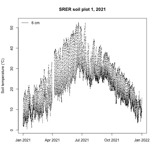
We see the expected pattern of warmer soil temperatures in the summer and cooler temperatures in the winter along with the typical diurnal cycles.
4. Soil water content
Now let's take a look at soil water content in the same plot, at the same depth. The soil water content data product page tells us that there is currently a problem with the sensor depths in the sensor_positions table in the soil water content data product and that we should instead use a file called swc_depthsV3.csv (downloadable on the linked page, under Documentation) to identify the correct depths. Depths are not currently displayed correctly in the sensor_positions table due to an unconventional data structure; future upgrades to the data processing pipeline will resolve this problem.
Looking at the row in the swc_depthsV3 file with siteID = SRER, horizontalPosition.HOR = "001" (soil plot 1), and verticalPosition.VER = "501" (measurement level 1) we see that the measurement depth was -0.06 m (i.e., 6 cm below the soil surface). So vertical position 501 is the depth we want.
Note that we do not expect the vertical index to correspond to the same depth in different data products (or different sites, or different plots). It's just an index, and in this particular set of soil water content data 501 corresponds to 6 cm, while in soil temperature 502 corresponded to 6cm.
We'll subset the soil water content data to soil plot 1 (horizontalPosition = "001"), with a nominal depth of 6 cm (verticalPosition = "501"), and that passed the QA/QC tests (VSWCFinalQF = 0).
soilWsub <- swc$SWS_30_minute |>
  filter(horizontalPosition=="001" &
           verticalPosition=="501" &
           VSWCFinalQF==0)
Let's create a time series plot of soil water content.
labelM=expression(paste("Soil water content (m"^" 3", " m"^"-3", ")"))

ggW <- ggplot(soilWsub, aes(startDateTime,
                            VSWCMean)) +
  geom_point(shape=".") +
  xlab("") +
  ylab(labelM)

ggW + ggtitle("SRER soil plot 1, 6cm depth, 2021")
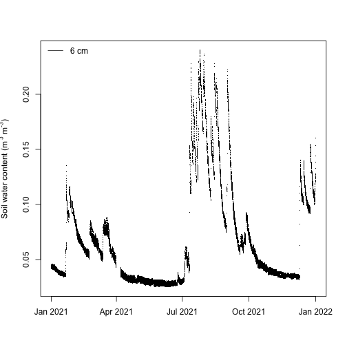
Soil water content shows typical patterns of sharp rises in moisture (presumably from rain events) followed by gradual declines as the soil dries. Soil moisture has a bimodal distribution being higher during winter and late summer, which is consistent with meteorology at SRER with winter rain as well as late summer thunderstorms.
5. Soil CO2 concentration
Now we want to see the temporal patterns in soil CO2 concentration data. Soil CO2 concentration is measured at three depths in surface soils in each soil plot and we'll look at data from all three depths. As we did with soil temperature and soil water content, we'll first subset to soil plot 1 measurements that passed the QA/QC tests (finalQF = 0). In this case we'll look at all three measurement depths: 501, 502, and 503.
soilCO2sub <- co2$SCO2C_30_minute |>
  filter(horizontalPosition=="001" &
           finalQF==0)
Next let's find out the depths of these measurements by looking up the rows corresponding to soil plot 1 in the sensor_positions table.
co2$sensor_positions_00095 |>
  filter(grepl("001[.]", HOR.VER)) |>
  select(HOR.VER, zOffset)

##   HOR.VER zOffset
## 1 001.501   -0.02
## 2 001.502   -0.05
## 3 001.503   -0.19
The sensors were measuring at 2, 5, and 19 cm below the soil surface.
Let's plot a time series of CO2 at each depth.
soilCO2sub <- soilCO2sub |>
  mutate(depth = case_when(verticalPosition=="501" ~ "2 cm",
                           verticalPosition=="502" ~ "5 cm",
                           verticalPosition=="503" ~ "19 cm"))


ggC <- ggplot(soilCO2sub, aes(startDateTime,
                             soilCO2concentrationMean)) +
  geom_point(shape=".", aes(color=depth)) +
  xlab("") +
  ylab("Mean soil CO2 concentration")

ggC
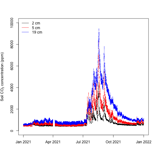
Soil CO2 concentrations were higher in the late summer and early fall and close to atmospheric levels in the winter through to early summer, reflecting the seasonal cycle of root, microbial and other soil organism activity. The typical soil CO2 concentration depth profile is also clear, with higher concentrations deeper in the soil reflecting the long time it takes CO2 produced at depth to diffuse to the atmosphere relative to CO2 produced near the soil surface.
6. Displaying the time series together
Now we've created separate time series plots for soil temperature, water content, and soil CO2 concentration. However, to help us looks for relationships between the three data sets it can be useful to plot them all on a single multi-panel plot.
grid.arrange(ggT, ggW,
             ggC + theme(legend.position="none"),
  nrow=3)
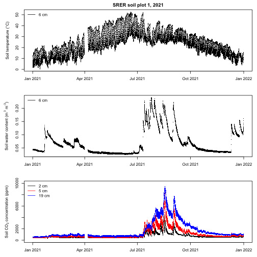
This multi-panel plot suggests that both soil temperature and water content influence soil CO2 concentrations at SRER. Specifically, soil CO2 concentrations tend to be low when the soil is cool regardless of water content, likewise concentrations tend to be low when the soil is dry regardless of temperature. When the soil is warm, CO2 concentrations responds rapidly to increases in soil moisture and then gradually decrease as the soil dries, presumably due to changes in the activity of roots and soil organisms.
In this tutorial we've focused on soil CO2 concentrations but most researchers are more interested in soil respiration rates than the soil CO2 concentrations themselves. Soil respiration can be calculated using these data products in combination with other NEON products, but this requires calculation of the soil CO2 diffusivity coefficient which is too complex to include in a brief data skills tutorial. There is a code package available in R, neonSoilFlux, developed by researchers in the NEON community to make these calculations. Consult the package and its documentation if you are interested in soil respiration.