Building Vegetation Model Initial Conditions from Field and Remote Sensing Data

Workshop Overview

Initializing the FATES Model using NEON Remote Sensing Data

Plants influence carbon storage, water and energy exchange, habitat, and competition within ecosystems. To represent those processes in an ecosystem model, we need more than a list of species: we need to know how much vegetation is present, which plant functional types (PFTs) they are, and how that vegetation is arranged across the landscape.

In this tutorial, you will use field observations (tree inventory) and airborne remote sensing data from the National Ecological Observatory Network (NEON) to build those descriptions for the Lower Teakettle site (TEAK) in California. The final products are initial-condition files for FATES, the Functionally Assembled Terrestrial Ecosystem Simulator.

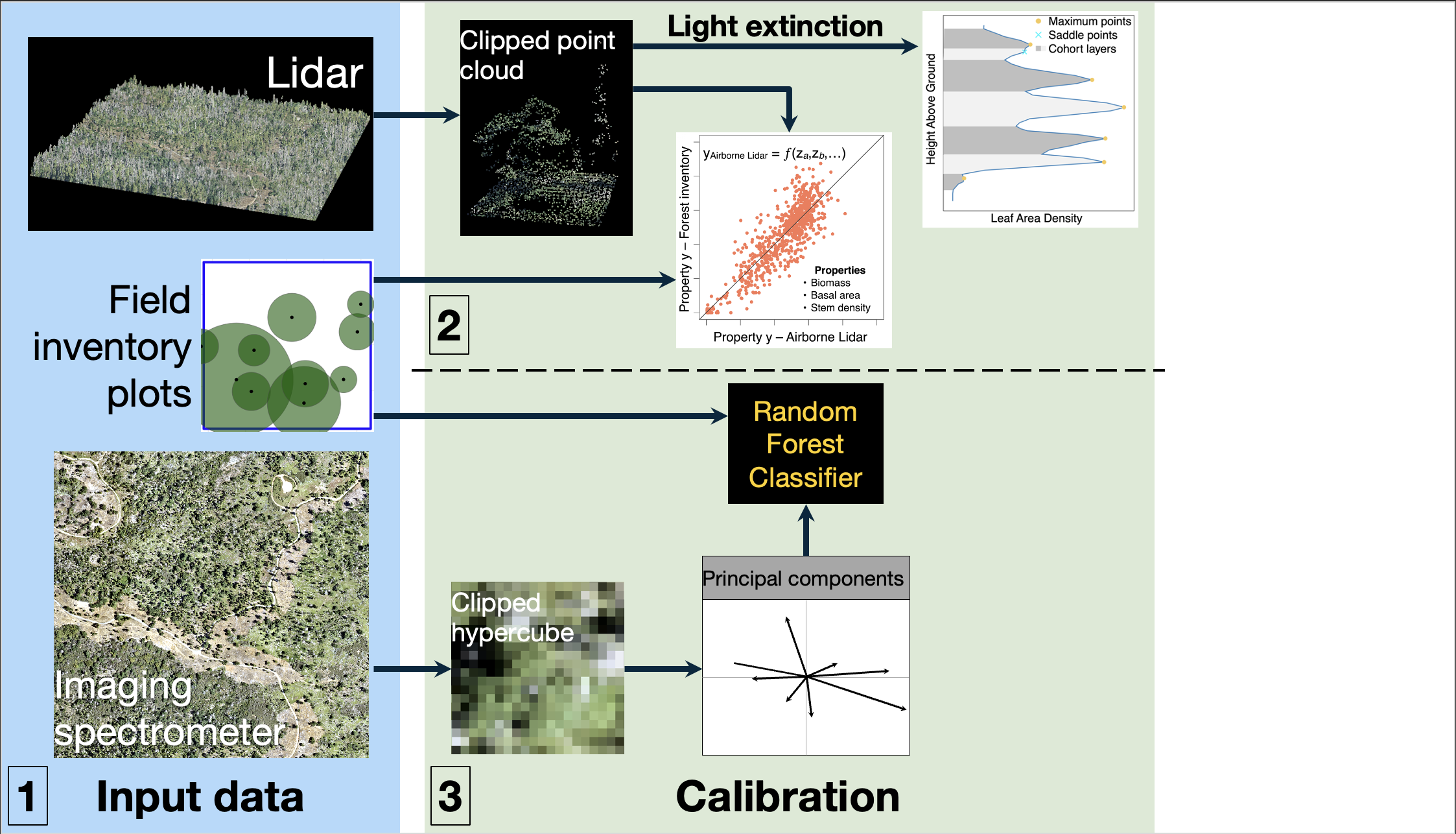
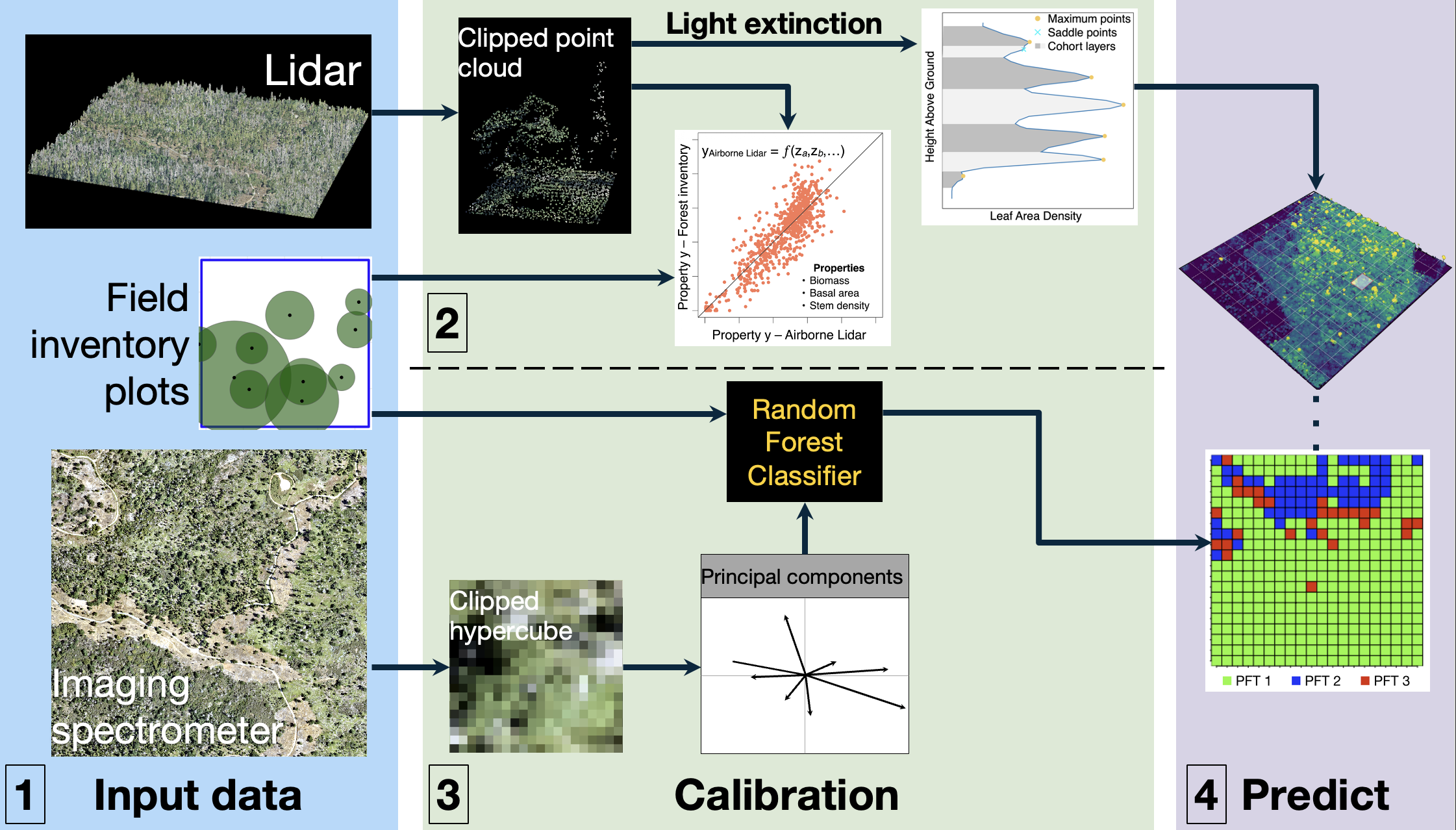
The notebook demonstrates a smaller-scale version of the PRISMATIC pipeline. This notebook walks through the PRISMATIC pipeline to use plot-based and remote sensing forest data to generate initial conditions for the FATES (Functionally Assembled Terrestrial Ecosystem Simulator) vegetation model. The main steps in the workflow are:

1. Download and clean NEON remote sensing and forest inventory data.
2. Develop a model to estimate vegetation size classes (height of canopy layers) calibrated by known tree sizes in forest inventory plots.
3. Develop a model to classify plant functional type (PFT) calibrated on known functional types in forest inventory plots.
4. Estimate size classes and PFTs across remote sensing extent to generate FATES initial conditions.

You can adapt the workflow to another NEON site, year, spatial extent, or PFTs.

Background: from observations to initial conditions for a process-based model

What is FATES?

FATES, the Functionally Assembled Terrestrial Ecosystem Simulator, is an open-source numerical model of terrestrial vegetation and ecosystem dynamics. It is primarily supported by the U.S. Department of Energy. FATES is implemented as a vegetation model that can be coupled to land-surface and Earth system modeling frameworks. Learn more in the open-source FATES GitHub repository and the FATES User's Guide.

To explain FATES briefly for the purposes of this tutorial, FATES represents vegetation by size and functional group. Plants are grouped as plant functional types (PFTs) that differ in traits relevant to growth, resource use, disturbance response, etc. Within a spatial unit of shared disturbance history, or patch, plants are further organized into cohorts, plants of the same PFT with similar size. Cohorts compete for light, water, and nutrients.

FATES can be initialized with known size and functional groups of vegetation describing the patches and cohorts. The PRISMATIC workflow helps construct those initial conditions from remote sensing data, calibrated by field observations. Lidar describes cohort structure, and lidar + hyperspectral imagery are used in classifying functional composition.

The model is the destination of this workflow, not the remote-sensing classifier itself. A PFT map or biomass raster is an intermediate ecological product; the cohort and patch files translate those products into the data structures that FATES can use to begin a simulation.

Why this matters

Observation-informed initialization can help researchers investigate how variation in forest composition, structure, and disturbance history affects modeled carbon cycling and vegetation change.

Study design

This workshop uses one 1 km x 1 km remote-sensing tile from NEON's Lower Teakettle (TEAK) site from 2021, however the whole workflow allows for entire site, multi-site, and multi-year implementation. Changing configuration values or forcing a rerun lets you explore how workflow choices affect the result.

Why combine field data and remote sensing?

Field inventory data give detailed information about individual stems, but these data are sparse, labor-intensive to collect, and may not represent the full variation of a landscape. Airborne observations provide broad spatial coverage.

The PRISMATIC strategy is therefore a supervised, observation-to-model workflow. It uses field measurements to define and calibrate plant functional type classification and forest structure.

Keep this question in mind throughout the notebook: What ecological information is being measured directly, what is being estimated, and how is uncertainty introduced at each handoff?

For additional project motivation and context, see the workshop background presentation.

import os

token = os.environ["NEON_API_TOKEN"]

Setup

Here we load the PRISMATIC modules which are Python and R scripts. The hydra module establishes the Hydra configuration, which sets the study site and years, identifies the raw, intermediate, and final data locations, and exposes parameters that control the analysis.

The step() helper wraps each pipeline function with the workflow's cache and rerun logic, which is helpful in a live workshop.

import sys, os
sys.path.insert(0, '..')

from hydra import initialize, compose
from omegaconf import OmegaConf

from utils.utils import build_cache_site, force_rerun
from initialize.inventory import download_veg_structure_data, download_trait_table, prep_veg_structure
from initialize.plots import download_polygons, prep_polygons
from initialize.lidar import download_lidar, download_aop_bbox, normalize_laz, clip_lidar_by_plots
from initialize.lad import prep_lad
from initialize.biomass import prep_biomass
from initialize.hyperspectral import (download_hyperspectral, correct_flightlines,
                                      prep_manual_training_data, prep_aop_imagery,
                                      extract_spectra_from_polygon, train_pft_classifier)
from initialize.generate_initial_conditions import generate_initial_conditions

with initialize(config_path='conf', version_base=None):
    cfg = compose(config_name='config')

site = 'TEAK'
year = '2021'
site_cfg = cfg.sites.run[site][year]
year_aop = site_cfg.year_aop

print(OmegaConf.to_yaml(site_cfg))

# --- Values from the Hydra config (the same ones main.py pulls out) ---
data_raw_aop_path = cfg.paths.data_raw_aop_path
data_raw_inv_path = cfg.paths.data_raw_inv_path
data_int_path     = cfg.paths.data_int_path
data_final_path   = cfg.paths.data_final_path

ic_type          = cfg.others.ic_type
hs_type          = cfg.others.hs_type
month_window     = cfg.others.month_window
n_plots          = cfg.others.n_plots
plot_length      = cfg.others.plot_length
ntree            = cfg.others.ntree
min_distance     = cfg.others.min_distance
use_tiles_w_veg  = cfg.others.use_tiles_w_veg
randomMinSamples = cfg.others.randomMinSamples
aggregate_from_1m_to_2m_res = cfg.others.aggregate_from_1m_to_2m_res
independentValidationSet    = cfg.others.independentValidationSet
pcaInsteadOfWavelengths     = cfg.others.pcaInsteadOfWavelengths
multisite        = cfg.others.multisite
coords_bbox      = cfg.others.coords_bbox
neon_trait_link  = cfg.others.neon_trait_table.neon_trait_link

use_case = "train"

# step(): run a pipeline function only if its outputs aren't already on disk.
# This mirrors main.py's force_rerun/cache wiring, so re-running a cell skips work
# that is already done and returns the existing output path(s) instead.
rerun_status = {k: bool(v) for k, v in site_cfg.force_rerun.items()}

def step(fn, **kwargs):
    cache = build_cache_site(site=site, year_inventory=year, year_aop=year_aop,
                             data_raw_aop_path=data_raw_aop_path,
                             data_raw_inv_path=data_raw_inv_path,
                             data_int_path=data_int_path,
                             hs_type=hs_type, coords_bbox=coords_bbox)
    return force_rerun(cache, force=rerun_status)(fn)(**kwargs)

1. Download and clean data

1a. Download data

Functions: download_veg_structure_data, download_polygons, download_trait_table, download_lidar, download_hyperspectral

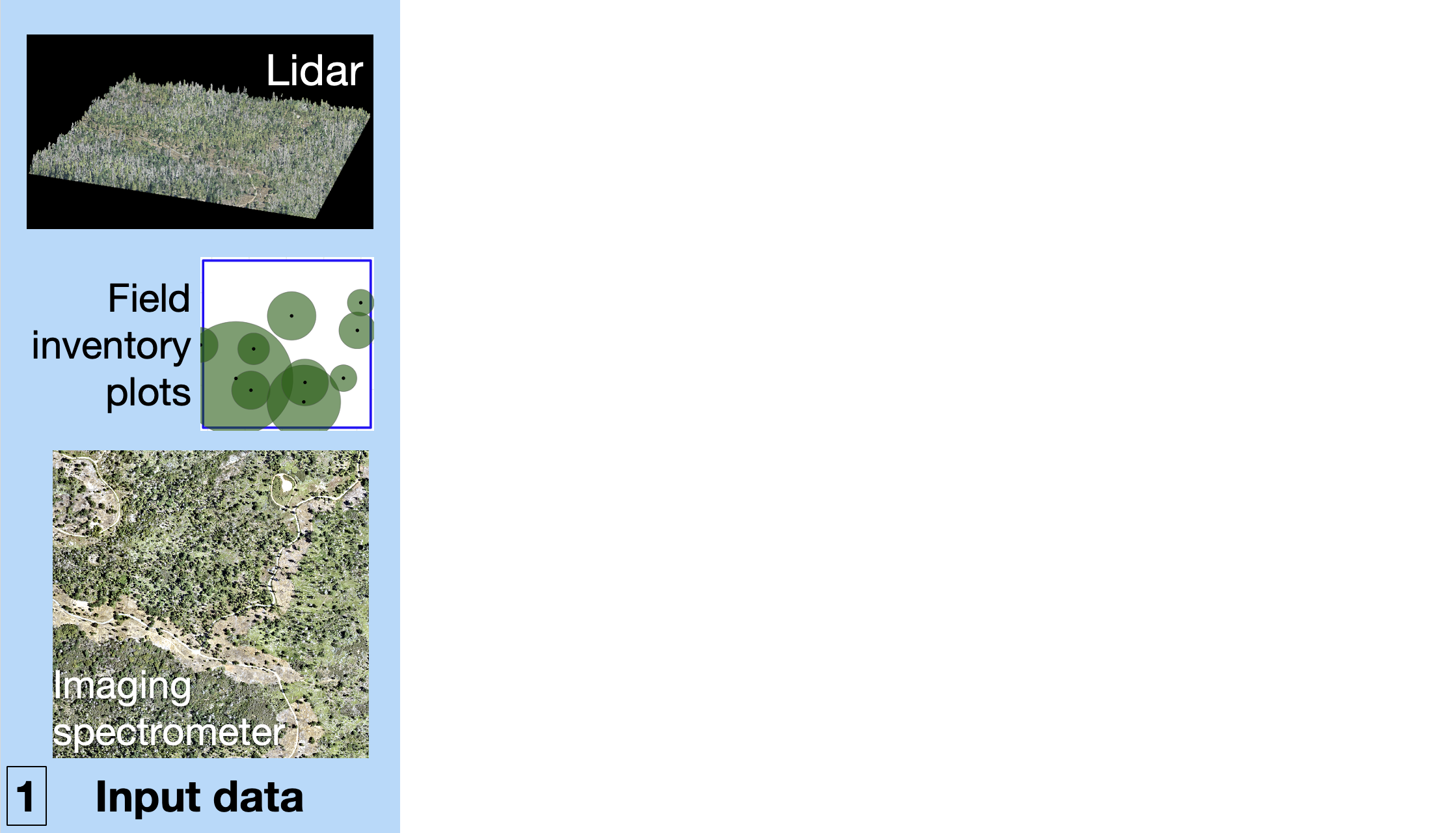
This step gathers the NEON remote sensing and forest inventory data that support later steps. Stem-level inventory records (DP1.10098.001) include species or taxonomic identity, diameter at breast height (DBH), height, and location. Plot polygons and sampling-effort information provide the footprint and sampling context of those measurements. The trait table provides attributes needed by the allometric biomass equations used later, and NEON's Airborne Observation Platform (AOP) supplies lidar and hyperspectral coverage for the same site and flight period.

NEON data products used:

• DP1.10098.001 │ Vegetation structure (woody plant measurements)
• DP3.30010.001 │ High-resolution orthorectified camera imagery (RGB)
• DP3.30006.001 │ Hyperspectral reflectance
• DP3.30026.001 │ Vegetation indices
• DP1.30003.001 │ Discrete return LiDAR point cloud
• DP3.30024.001 │ Digital Terrain Model (DTM)
• DP3.30025.001 │ Slope and aspect
• DP3.30015.001 │ Ecosystem structure / Canopy Height Model (CHM)

from initialize.inventory import download_veg_structure_data, download_trait_table
from initialize.plots import download_polygons

# Download stem-level vegetation structure data (species, DBH, height, location)
download_veg_structure_data(cfg, site, year)

# Download NEON plot boundary polygons
download_polygons(cfg, site, year)

# Download NEON trait table (used later for allometric biomass equations)
download_trait_table(cfg)

from initialize.lidar import download_lidar, download_aop_bbox
from initialize.hyperspectral import download_hyperspectral

# Download LiDAR point clouds (.laz files) for the site/year
# Use download_aop_bbox to restrict to a spatial bounding box if needed
download_lidar(cfg, site, year)

# Download hyperspectral flightline imagery
download_hyperspectral(cfg, site, year)

1b. Clean forest inventory data

Functions: prep_veg_structure, prep_polygons

Filter inventory records to the target year and to a configurable time window around the AOP flight. This temporal match matters because a forest can change between the field survey and the airborne observation. It also assigns PFT labels to individual plants and partitions plot polygons into spatial subunits that can be paired with remote-sensing pixels.

from initialize.inventory import prep_veg_structure
from initialize.plots import prep_polygons

# Filter stems to target year, assign PFT labels
prep_veg_structure(cfg, site, year)

# Partition plot polygons into spatial subunits for RS linking
prep_polygons(cfg, site, year)

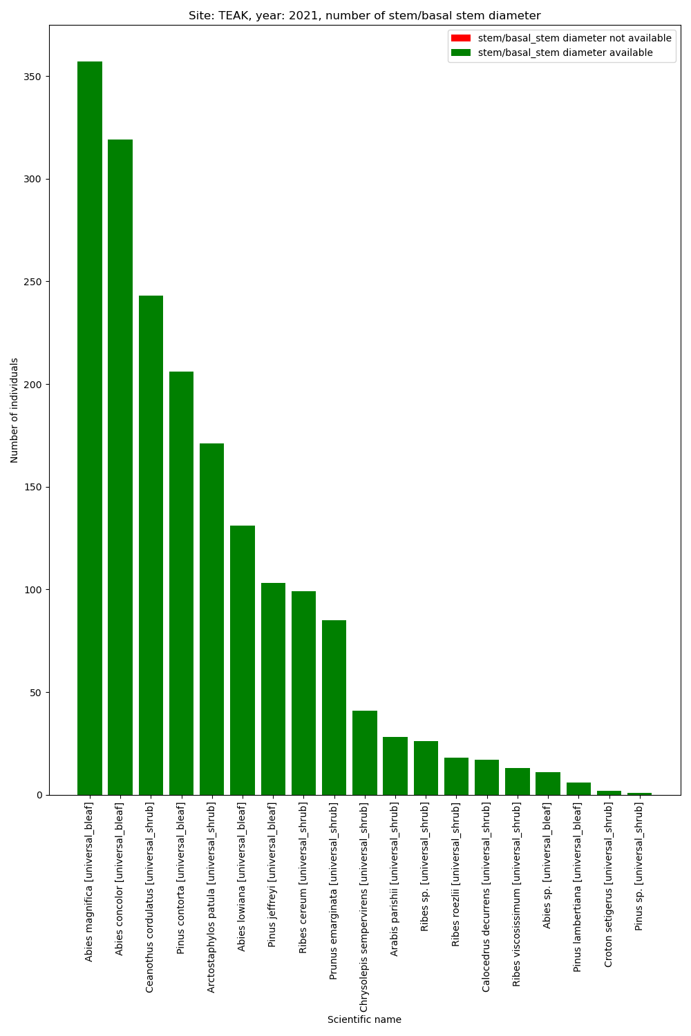
Count of taxonomic types in NEON forest inventory plots at TEAK in 2021

2. Develop a size model

2a. Processing lidar: Normalization and Clipping

Functions: normalize_laz, clip_lidar_by_plots

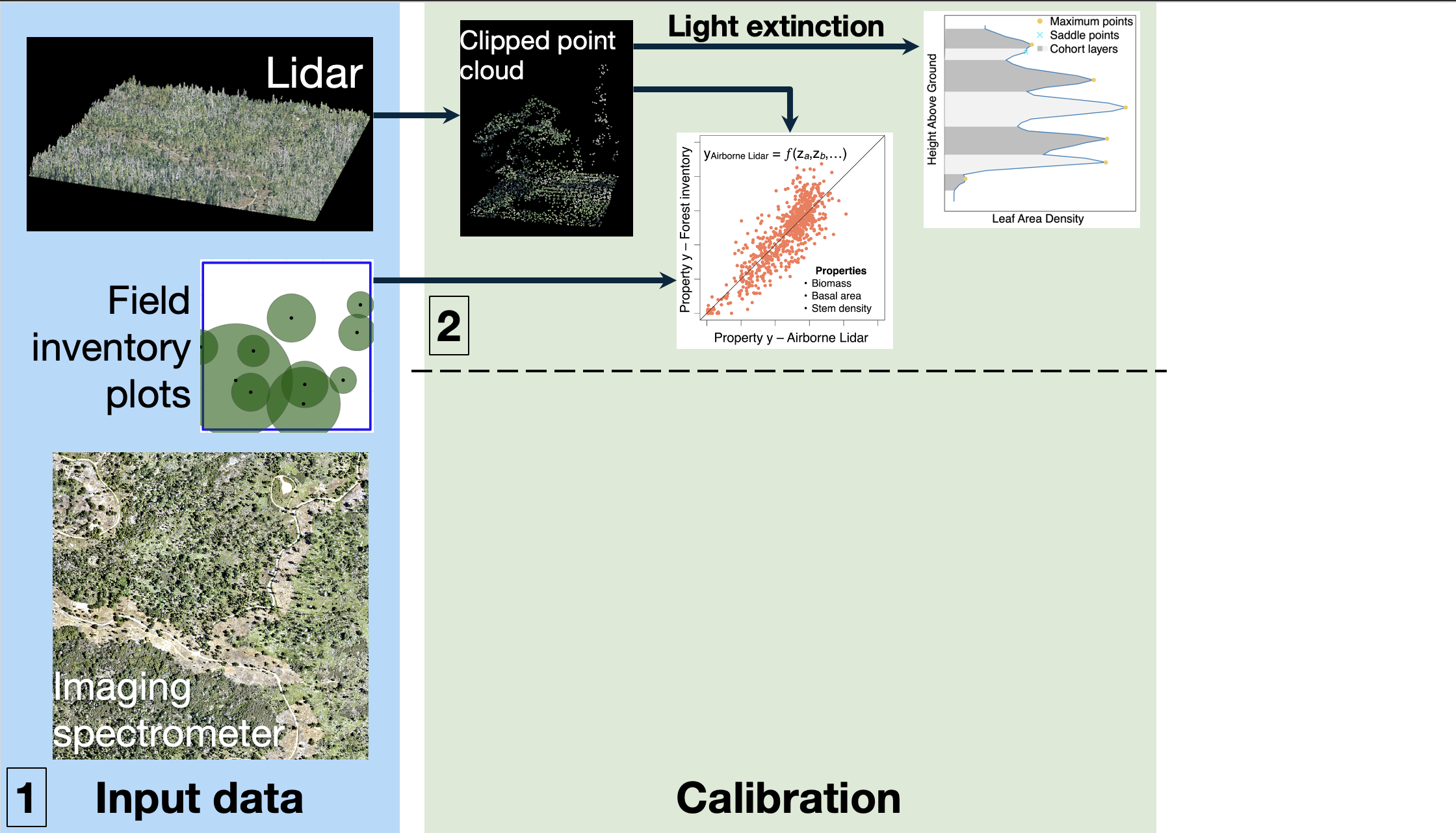
Lidar is a three-dimensional point cloud. Each point has an absolute (x,y,z) coordinate in space and we normalize it to get a normalized (x,y,zn) coordinate for the point height above ground.

The normalized point cloud is then clipped to the partitioned plot boundaries. This is the key spatial join between airborne structure and field observations: the lidar points used to characterize a plot are drawn from the same area in which the inventory was collected.

Expected product: normalized, plot-clipped lidar point clouds suitable for deriving vertical canopy metrics.

from initialize.lidar import normalize_laz, clip_lidar_by_plots

# Subtract digital terrain model so z reflects canopy height above ground
normalize_laz(cfg, site, year)

# Clip normalized point clouds to NEON plot boundaries
clip_lidar_by_plots(cfg, site, year)

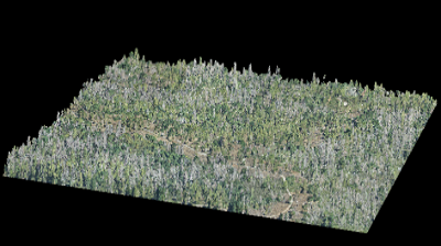
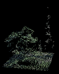
Left, 1 km2 NEON AOP normalized lidar tile point cloud. Right, lidar point cloud clipped to plot extent

2b. Deriving Canopy Structure: Leaf Area Density Profiles

Function: prep_lad

Leaf area density (LAD) describes how leaf area is distributed vertically through the canopy. A LAD profile tells us where vegetation is concentrated, how many canopy layers are present, and how dense those layers are. Local maxima in a profile provide candidate canopy layers. These layers are used to define FATES cohort heights, because FATES represents plants of similar height as cohorts that occupy comparable light environments.

from initialize.lad import prep_lad

# Compute LAD profiles per plot, stratified by PFT size class
prep_lad(cfg, site, year)

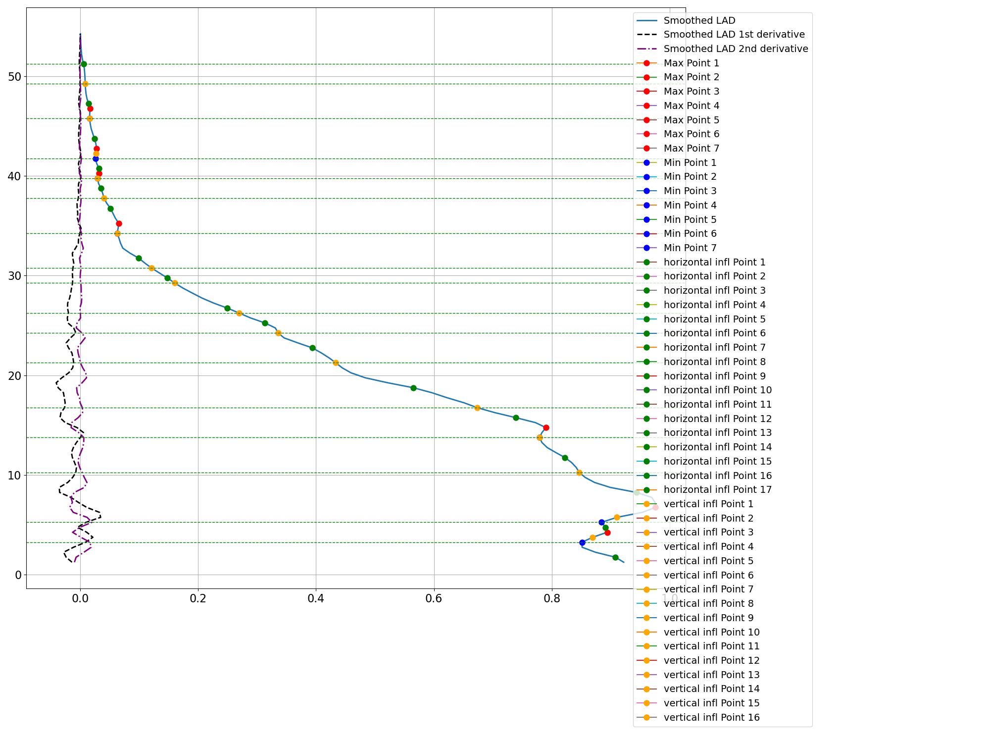
Leaf area density profile for a plot. Local maxima mark candidate size classes used to define FATES cohorts.

2c. Estimating Biomass

Function: prep_biomass

The inventory contains measurements such as DBH and height, but biomass is not measured directly for every living stem. PRISMATIC applies species- or trait-informed allometric equations to estimate above-ground biomass. These equations use observable stem dimensions together with the NEON trait table to convert field measurements into biomass.

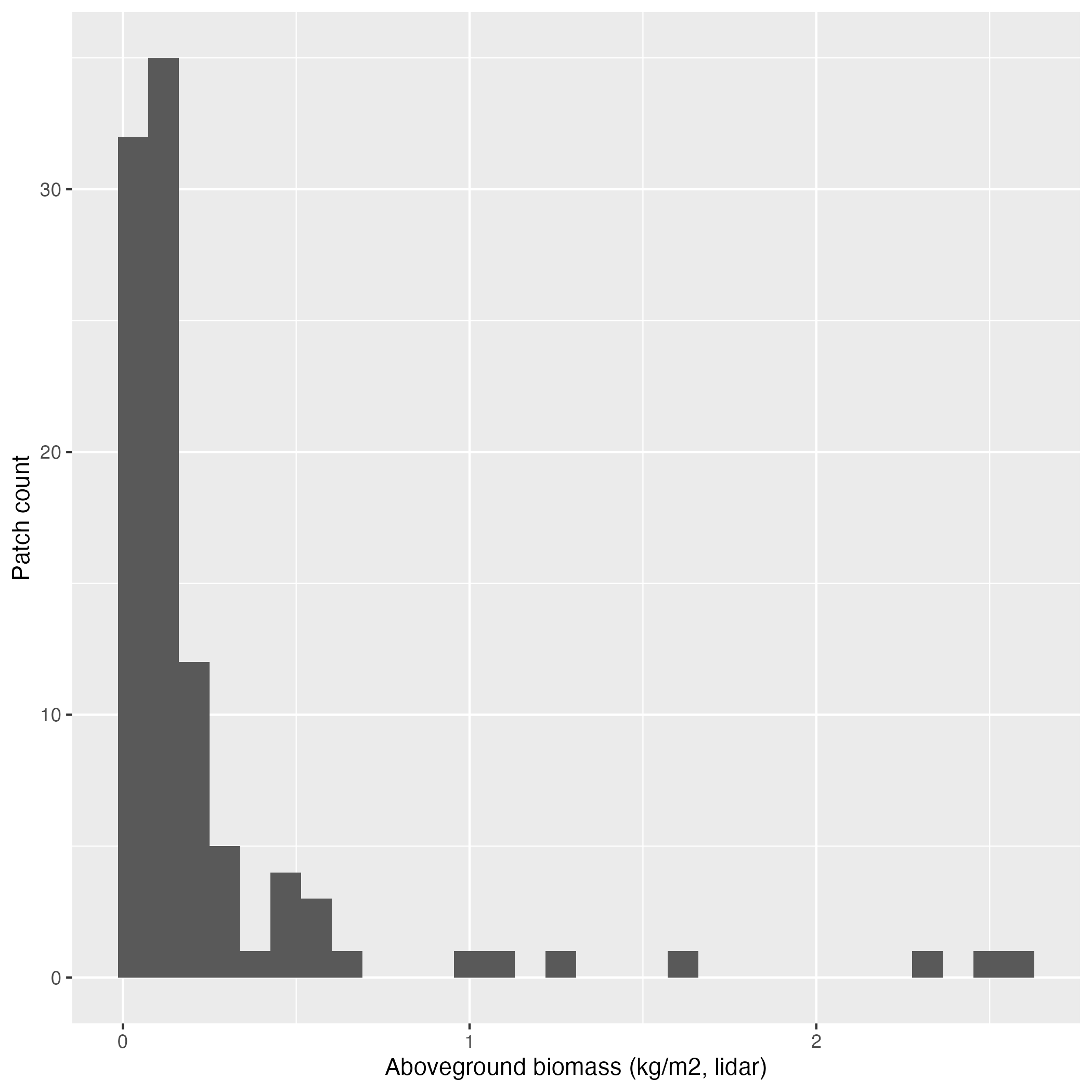
Biomass is summarized by plot and PFT and is carried into the final FATES initialization. The workflow also derives related community measurements, including stem density, basal area, and biomass per plot. These summaries can be used to check whether the remote-sensing-based products remain ecologically plausible.

from initialize.biomass import prep_biomass

# Estimate AGB per stem using species-specific allometry from the NEON trait table
prep_biomass(cfg, site, year)

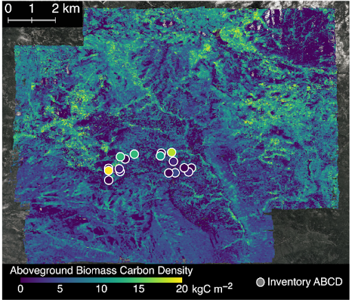
Example of biomass map generated across NEON SOAP site (also in California)

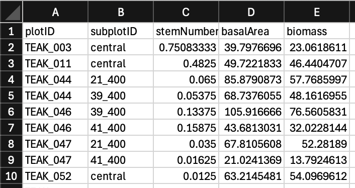
In this workflow we also calculate stem density, basal area, and biomass per plot

3. Develop plant functional type (PFT) classifier

3a. Preparing Hyperspectral Imagery

Functions: prep_aop_imagery

Hyperspectral imagery records reflectance in many narrow wavelength bands. Those bands contain information about leaf chemistry, pigments, water content, and canopy composition that can help distinguish functional types. lidar-derived rasters contribute complementary information about height and structure. We stack lidar-derived rasters (e.g. NDVI, DEM) and hyperspectral bands (e.g. PCA bands) to prepare the AOP-derived data as features in a random forest later in this step

from initialize.hyperspectral import prep_aop_imagery

# Stack corrected hyperspectral bands + LiDAR rasters into a single image
prep_aop_imagery(cfg, site, year)

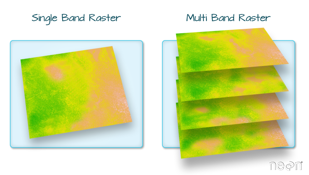
Visualization of the raster stack used as training data.

From https://www.neonscience.org/resources/learning-hub/tutorials/dc-multiband-rasters-r

3b. Building the Training Dataset

Functions: prep_manual_training_data, extract_spectra_from_polygon

A classifier needs examples for which both the predictor values and the correct class are known. PRISMATIC creates those examples by combining inventory-derived crown polygons with the stacked AOP raster. Pixels inside a labeled crown inherit the PFT assigned from the field data, while their feature values come from the hyperspectral and structural layers.

from initialize.hyperspectral import extract_spectra_from_polygon

# Extract per-pixel spectra within each crown polygon and attach PFT labels
extract_spectra_from_polygon(cfg, site, year)

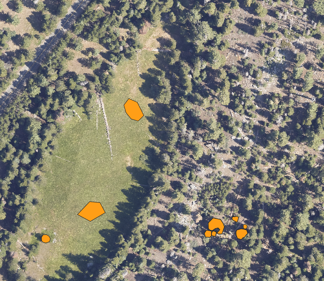
Screenshot of a few manually labelled polygons used as training data.

3c. Training the PFT Classifier

Function: train_pft_classifier

In this step we train a Random Forest classifier using the labeled spectra. A Random Forest combines many decision trees, each trained on a different resampled view of the data, to produce a prediction that can capture nonlinear relationships among wavelengths, structural layers, and PFT labels. Because hyperspectral data can contain many correlated bands, the configuration can use principal components instead of the original wavelengths.

The confusion matrix cross-tabulates predicted versus true PFT labels, so its off-diagonal entries show which pairs of PFTs are most often misclassified as one another; feature importance indicates which raster layers contribute most to predictions; and held-out or cross-validation agreement provides a measure of how consistently the model generalizes beyond the samples used to fit it.

In this tutorial, the classifier interface can support site-specific or multi-site training. Check the configuration and cached outputs when interpreting the result: a model trained across several NEON sites may transfer differently than one trained only on TEAK. If using a NEON site with new PFTs, the user will need to provide their own labelled crown polygons

from initialize.hyperspectral import train_pft_classifier

# Train Random Forest on labeled spectral data; evaluate with held-out accuracy
train_pft_classifier(cfg, site, year)

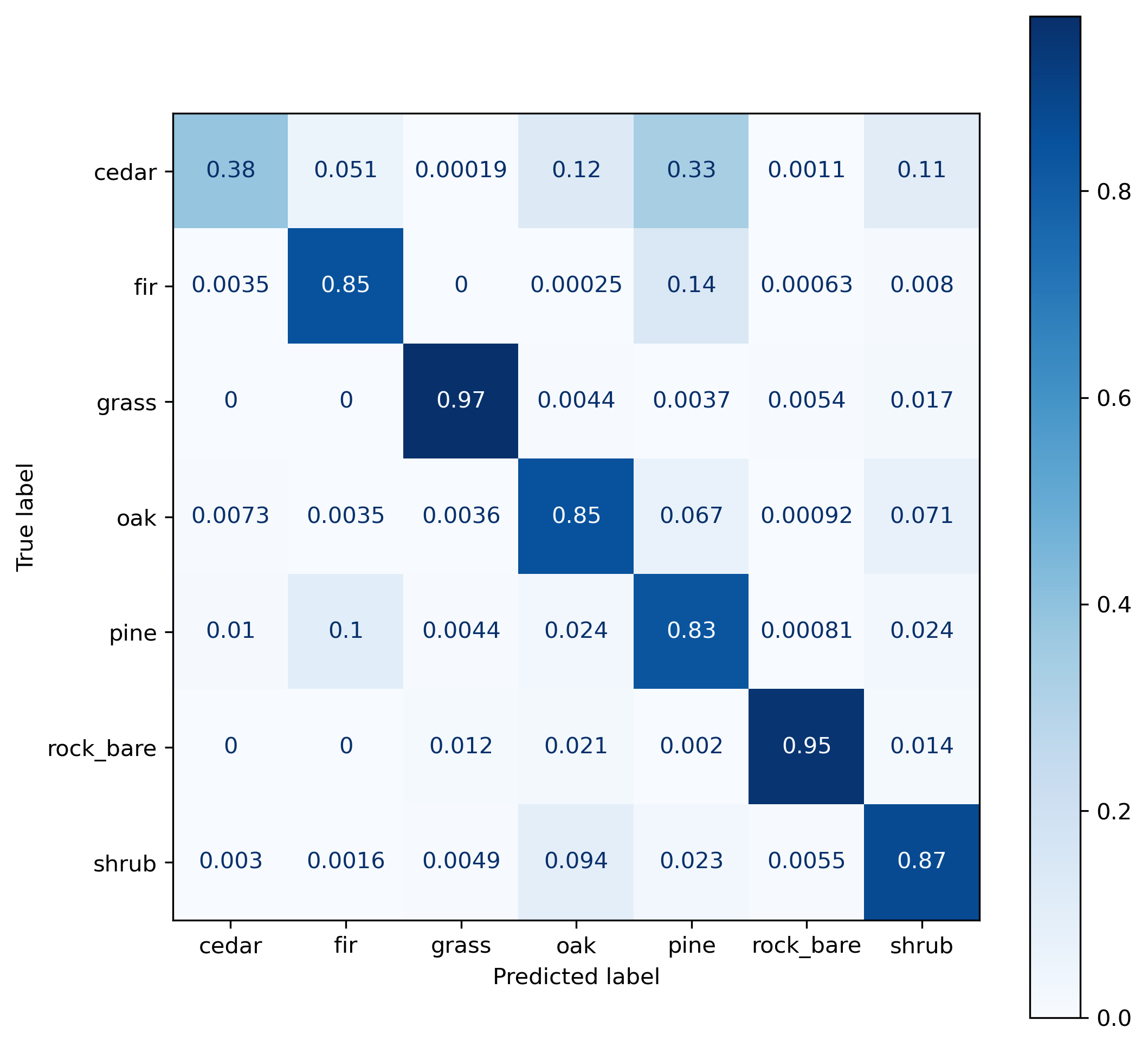
Confusion matrix of random forest performance on training data

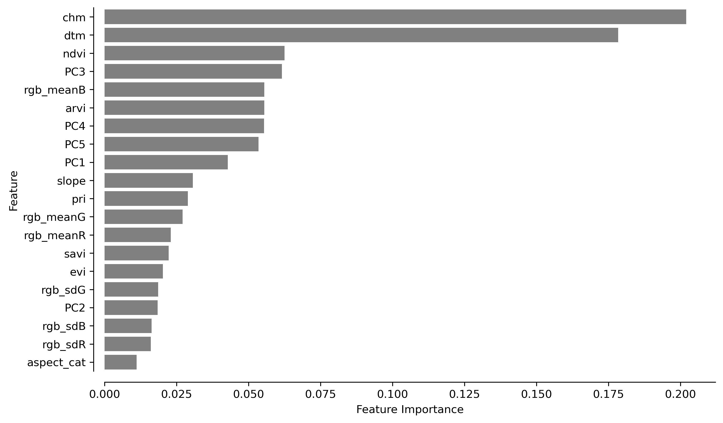
Rank of raster layers (or features) used in training in order of importance

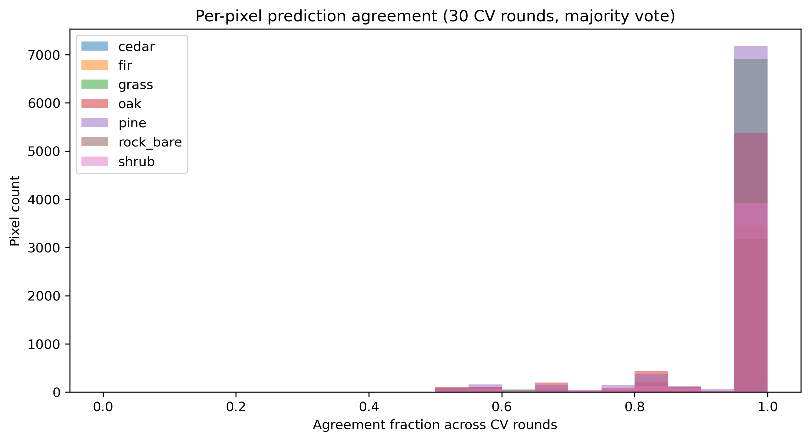
Per pixel agreement through k-fold cross-validation

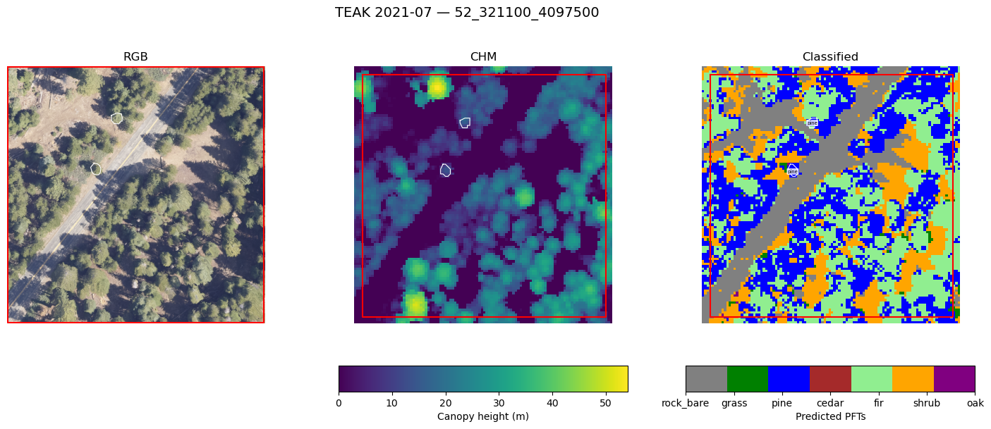
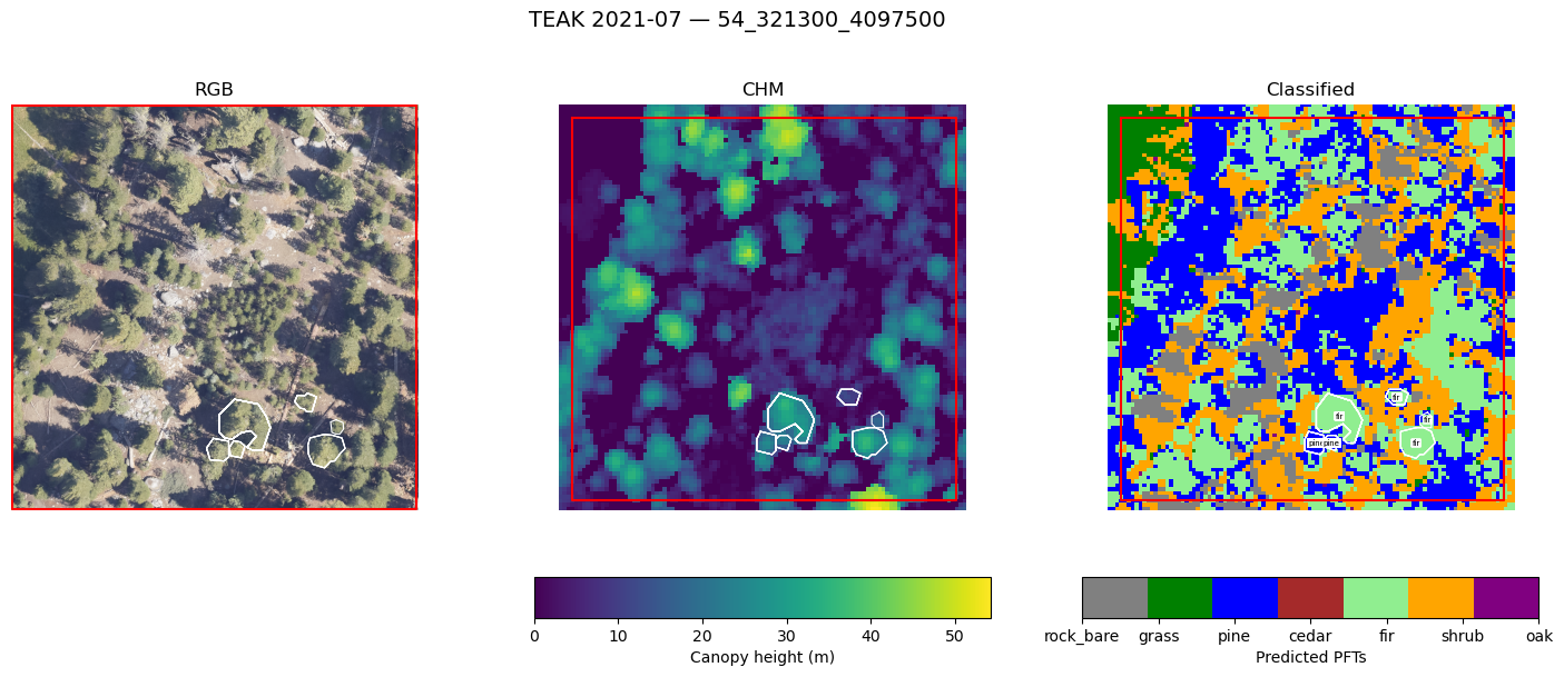
Two plots where we compare RGB, CHM, and classified PFT rasters.

4. Generate FATES initial conditions

Function: generate_initial_conditions

The trained classifier is applied wall-to-wall across the remote-sensing tile. PRISMATIC combines the resulting PFT map with canopy size classes. The result is no longer just a remote-sensing classification: it is a model-ready description of vegetation organized according to FATES's patch and cohort concepts.

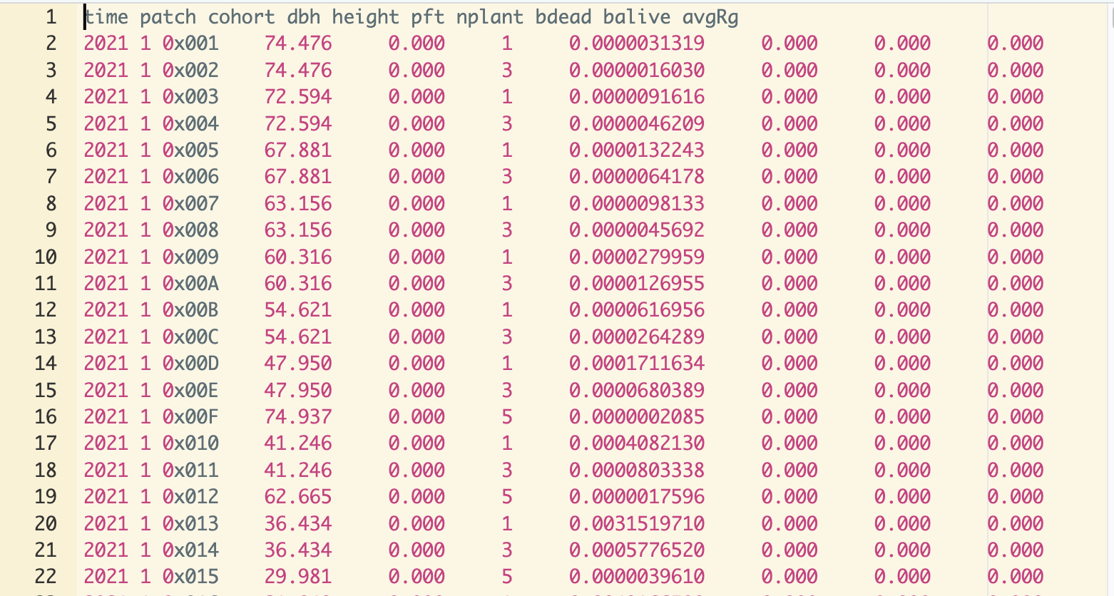
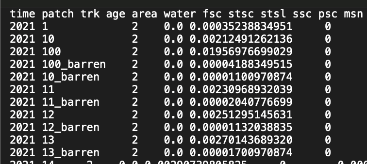
The final products are two space-delimited files:

• The cohort file describes the cohorts within each patch, including their PFT identity, height or size class, and associated vegetation quantities.
• The patch file describes the patches that make up the modeled site and connects them to the cohort records.

from initialize.generate_initial_conditions import generate_initial_conditions

# Classify wall-to-wall, aggregate to cohorts/patches, write FATES IC files
generate_initial_conditions(cfg, site, year)

Cohort file example

Patch file example

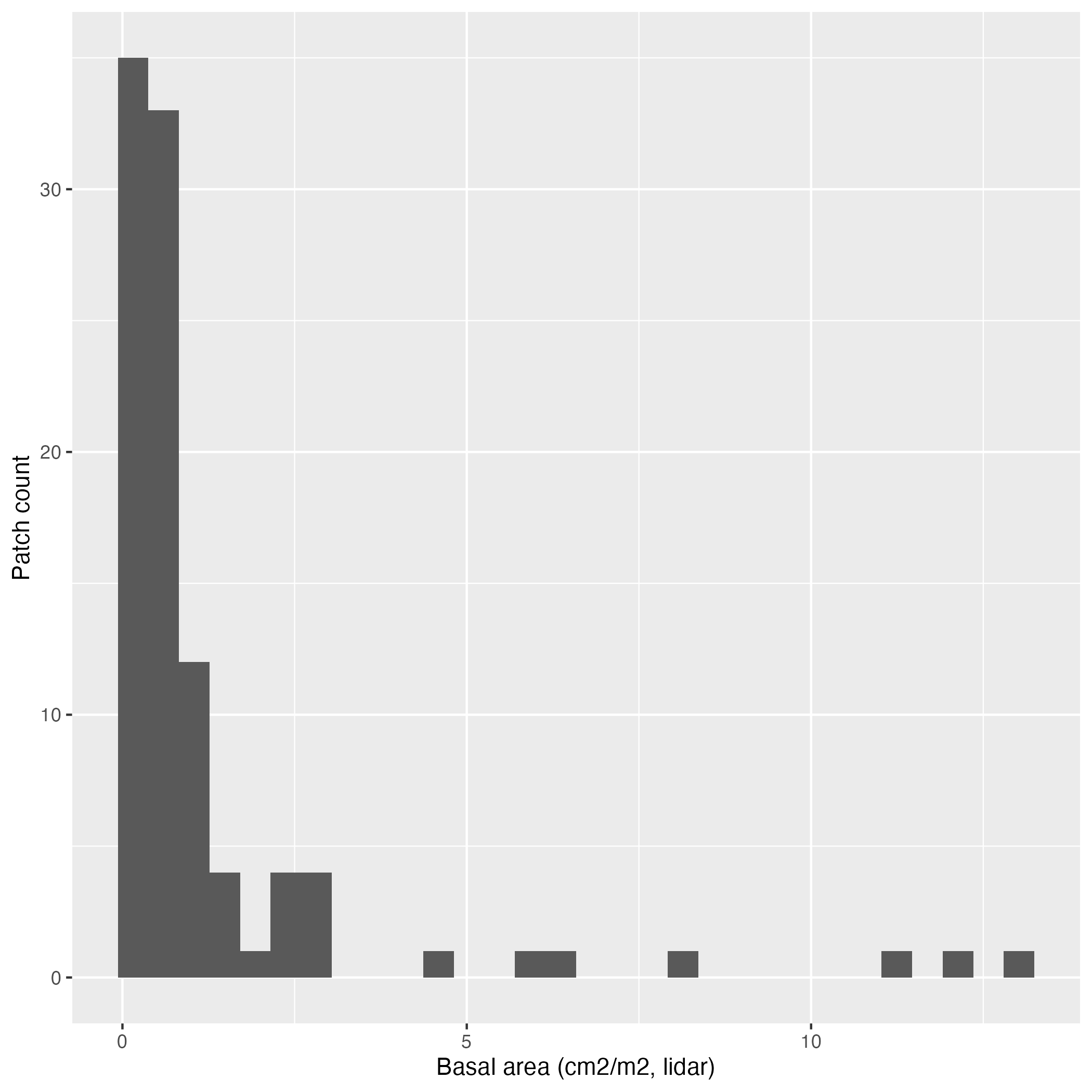
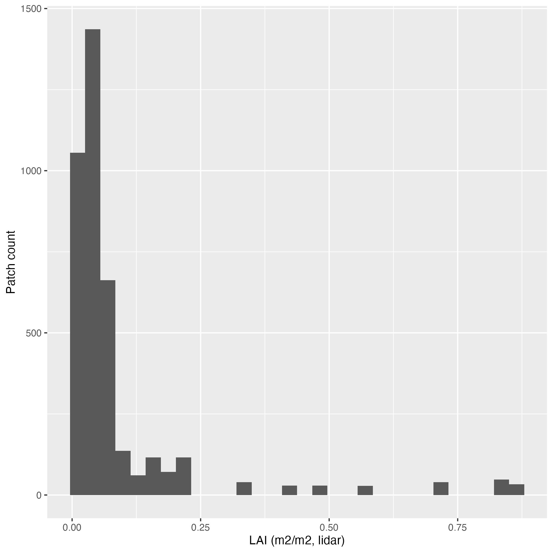
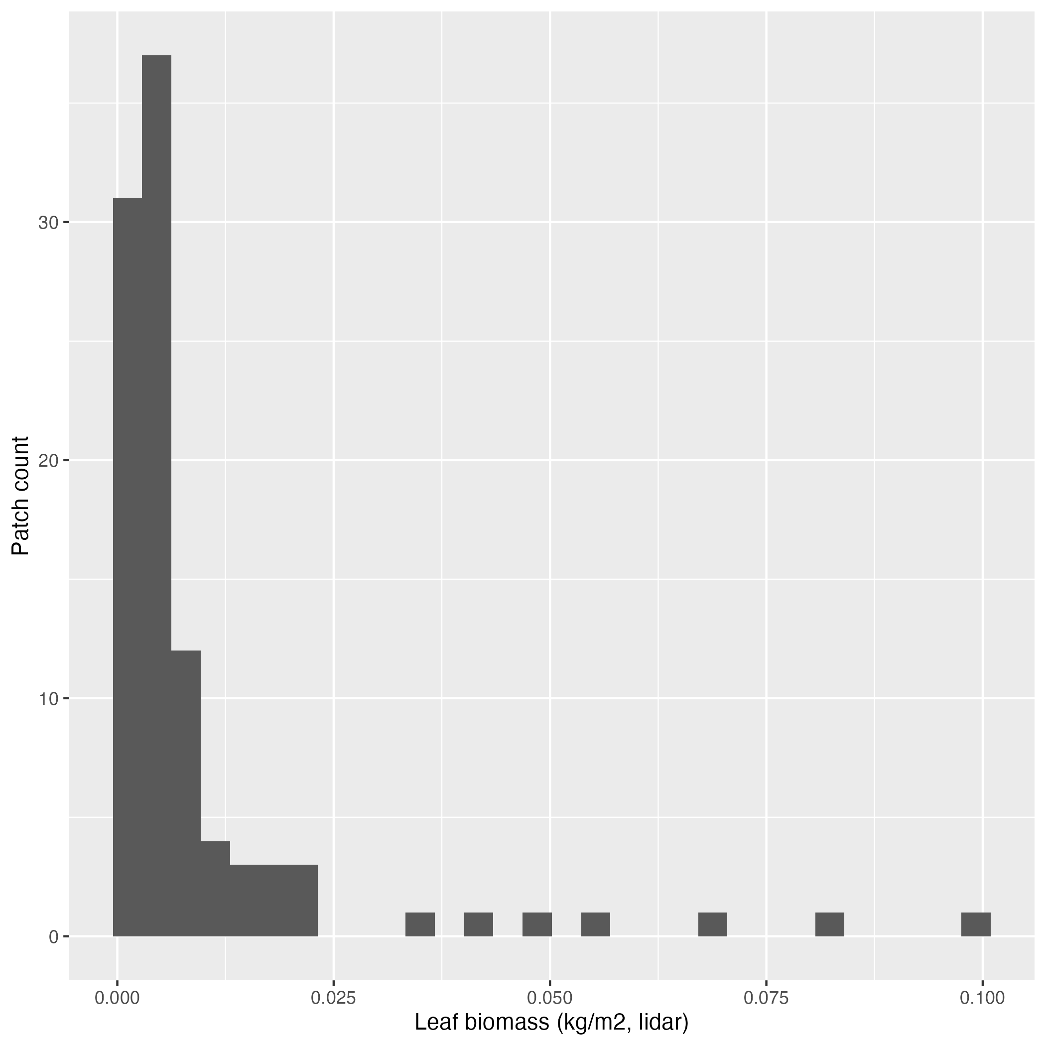
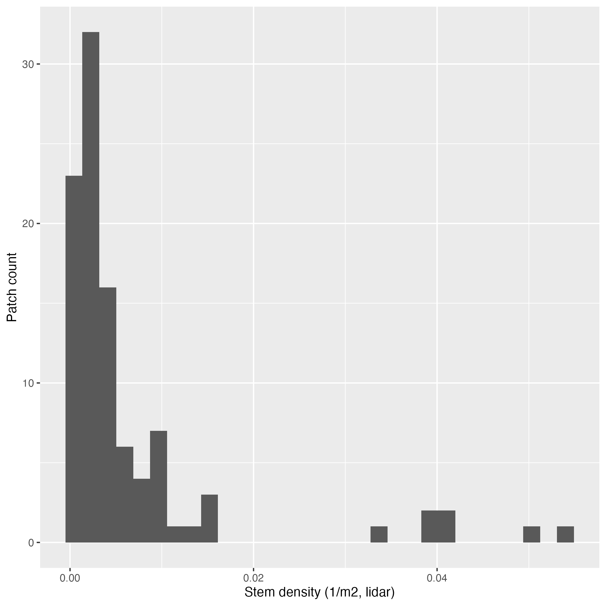
Summary community measurements across this TEAK AOP tile

5. Where We're Going: FATES Simulations

The patch and cohort files generated above are inputs, not the endpoint of the ecological analysis. FATES uses them to initialize a dynamic simulation in which cohorts grow, compete, reproduce, die, and respond to disturbance. Because the initialization contains spatially informed PFT composition and vertical structure, the simulation can begin from a community state grounded in observations.

Below are example outputs from FATES runs initialized with PRISMATIC data, showing how the spatially-informed PFT structure and size classes translate into simulated forest dynamics over time.

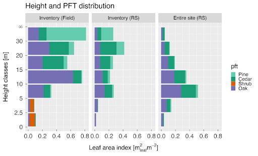
Comparison initial conditions from field and remote sensing sources.

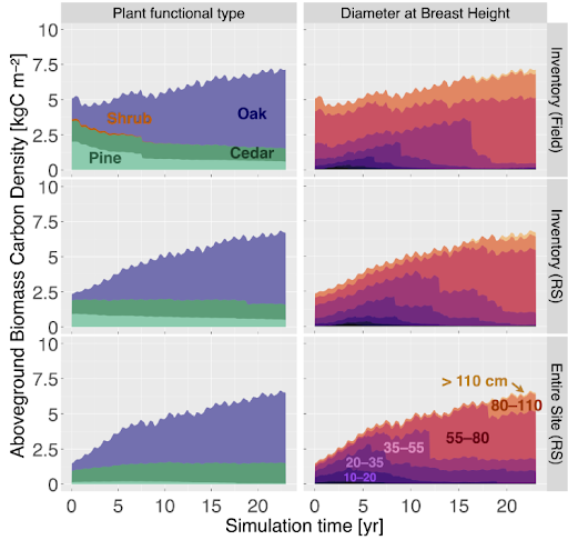
Visualization of FATES PFT distributions through time from varying initial conditions sources