Tutorial
Detecting Foggy Images using the hazer Package
Last Updated: Apr 2, 2026
In this tutorial, you will learn how to
- perform basic image processing and
- estimate image haziness as an indication of fog, cloud or other natural or artificial factors using the
hazerR package.
Read & Plot Image
We will use several packages in this tutorial. All are available from CRAN.
# load packages
library(hazer)
library(jpeg)
library(data.table)
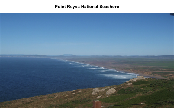
Before we start the image processing steps, let's read in and plot an image. This image is an example image that comes with the hazer package.
# read the path to the example image
jpeg_file <- system.file(package = 'hazer', 'pointreyes.jpg')

# read the image as an array
rgb_array <- jpeg::readJPEG(jpeg_file)

# plot the RGB array on the active device panel


# first set the margin in this order:(bottom, left, top, right)
par(mar=c(0,0,3,0))
plotRGBArray(rgb_array, bty = 'n', main = 'Point Reyes National Seashore')
When we work with images, all data we work with is generally on the scale of each individual pixel in the image. Therefore, for large images we will be working with large matrices that hold the value for each pixel. Keep this in mind before opening some of the matrices we'll be creating this tutorial as it can take a while for them to load.
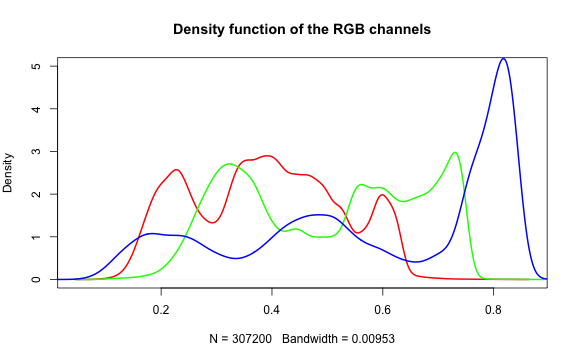
Histogram of RGB channels
A histogram of the colors can be useful to understanding what our image is made
up of. Using the density() function from the base stats package, we can extract
density distribution of each color channel.
# color channels can be extracted from the matrix
red_vector <- rgb_array[,,1]
green_vector <- rgb_array[,,2]
blue_vector <- rgb_array[,,3]

# plotting
par(mar=c(5,4,4,2))
plot(density(red_vector), col = 'red', lwd = 2,
		 main = 'Density function of the RGB channels', ylim = c(0,5))
lines(density(green_vector), col = 'green', lwd = 2)
lines(density(blue_vector), col = 'blue', lwd = 2)
In hazer we can also extract three basic elements of an RGB image :
- Brightness
- Darkness
- Contrast
Brightness
The brightness matrix comes from the maximum value of the R, G, or B channel. We
can extract and show the brightness matrix using the getBrightness() function.
# extracting the brightness matrix
brightness_mat <- getBrightness(rgb_array)

# unlike the RGB array which has 3 dimensions, the brightness matrix has only two
# dimensions and can be shown as a grayscale image,
# we can do this using the same plotRGBArray function
par(mar=c(0,0,3,0))
plotRGBArray(brightness_mat, bty = 'n', main = 'Brightness matrix')
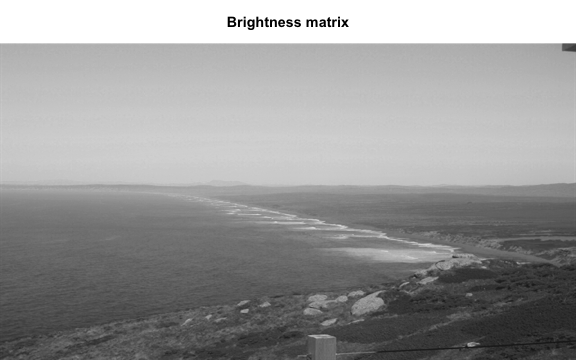
Here the grayscale is used to show the value of each pixel's maximum brightness of the R, G or B color channel.
To extract a single brightness value for the image, depending on our needs we can perform some statistics or we can just use the mean of this matrix.
# the main quantiles
quantile(brightness_mat)

#>         0%        25%        50%        75%       100%
#> 0.09019608 0.43529412 0.62745098 0.80000000 0.91764706


# create histogram
par(mar=c(5,4,4,2))
hist(brightness_mat)
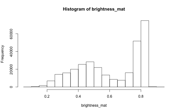
Why are we getting so many images up in the high range of the brightness? Where does this correlate to on the RGB image?
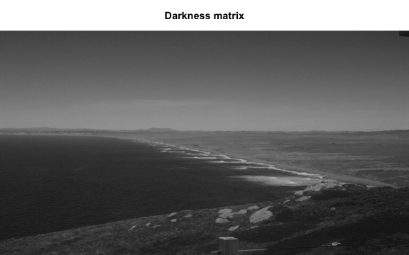
Darkness
Darkness is determined by the minimum of the R, G or B color channel.
Similarly, we can extract and show the darkness matrix using the getDarkness() function.
# extracting the darkness matrix
darkness_mat <- getDarkness(rgb_array)
# the darkness matrix has also two dimensions and can be shown as a grayscale image
par(mar=c(0,0,3,0))
plotRGBArray(darkness_mat, bty = 'n', main = 'Darkness matrix')
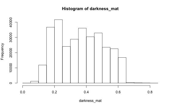
# main quantiles
quantile(darkness_mat)
#> 0% 25% 50% 75% 100%
#> 0.03529412 0.23137255 0.36470588 0.47843137 0.83529412
# histogram
par(mar=c(5,4,4,2))
hist(darkness_mat)
Contrast
The contrast of an image is the difference between the darkness and brightness of the image. The contrast matrix is calculated by difference between the darkness and brightness matrices.
The contrast of the image can quickly be extracted using the getContrast() function.
# extracting the contrast matrix
contrast_mat <- getContrast(rgb_array)

# the contrast matrix has also 2D and can be shown as a grayscale image
par(mar=c(0,0,3,0))
plotRGBArray(contrast_mat, bty = 'n', main = 'Contrast matrix')

# main quantiles
quantile(contrast_mat)

#>        0%       25%       50%       75%      100%
#> 0.0000000 0.1450980 0.2470588 0.3333333 0.4509804


# histogram
par(mar=c(5,4,4,2))
hist(contrast_mat)
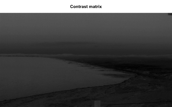
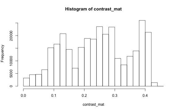
Image fogginess & haziness
Haziness of an image can be estimated using the getHazeFactor() function. This
function is based on the method described in
Mao et al. (2014).
The technique was originally developed to for "detecting foggy images and
estimating the haze degree factor" for a wide range of outdoor conditions.
The function returns a vector of two numeric values:
- haze as the haze degree and
- A0 as the global atmospheric light, as it is explained in the original paper.
The PhenoCam standards classify any image with the haze degree greater than 0.4 as a significantly foggy image.
# extracting the haze matrix
haze_degree <- getHazeFactor(rgb_array)

print(haze_degree)

#> $haze
#> [1] 0.2251633
#>
#> $A0
#> [1] 0.7105258
Here we have the haze values for our image. Note that the values might be slightly different due to rounding errors on different platforms.
Process sets of images
We can use for loops or the lapply functions to extract the haze values for
a stack of images.
You can download the related datasets from here (direct download).
Download and extract the zip file to be used as input data for the following step.
# to download via R
dir.create('data')

#> Warning in dir.create("data"): 'data' already exists

destfile = 'data/pointreyes.zip'
download.file(destfile = destfile, mode = 'wb', url = 'http://bit.ly/2F8w2Ia')
unzip(destfile, exdir = 'data')


# set up the input image directory
#pointreyes_dir <- '/path/to/image/directory/'
pointreyes_dir <- 'data/pointreyes/'

# get a list of all .jpg files in the directory
pointreyes_images <- dir(path = pointreyes_dir,
                         pattern = '*.jpg',
                         ignore.case = TRUE,
                         full.names = TRUE)
Now we can use a for loop to process all of the images to get the haze and A0 values.
(Note, this loop may take a while to process.)
# number of images
n <- length(pointreyes_images)

# create an empty matrix to fill with haze and A0 values
haze_mat <- data.table()

# the process takes a bit, a progress bar lets us know it is working.
pb <- txtProgressBar(0, n, style = 3)

#>
|
| | 0%
for(i in 1:n) {
  image_path <- pointreyes_images[i]
  img <- jpeg::readJPEG(image_path)
  haze <- getHazeFactor(img)

  haze_mat <- rbind(haze_mat,
                    data.table(file = image_path,
                               haze = haze[1],
                               A0 = haze[2]))

  setTxtProgressBar(pb, i)
}

#>
|
|= | 1%
|
|== | 3%
|
|=== | 4%
|
|===== | 6%
|
|====== | 7%
|
|======= | 8%
|
|======== | 10%
|
|========= | 11%
|
|========== | 13%
|
|============ | 14%
|
|============= | 15%
|
|============== | 17%
|
|=============== | 18%
|
|================ | 20%
|
|================= | 21%
|
|================== | 23%
|
|==================== | 24%
|
|===================== | 25%
|
|====================== | 27%
|
|======================= | 28%
|
|======================== | 30%
|
|========================= | 31%
|
|=========================== | 32%
|
|============================ | 34%
|
|============================= | 35%
|
|============================== | 37%
|
|=============================== | 38%
|
|================================ | 39%
|
|================================= | 41%
|
|=================================== | 42%
|
|==================================== | 44%
|
|===================================== | 45%
|
|====================================== | 46%
|
|======================================= | 48%
|
|======================================== | 49%
|
|========================================== | 51%
|
|=========================================== | 52%
|
|============================================ | 54%
|
|============================================= | 55%
|
|============================================== | 56%
|
|=============================================== | 58%
|
|================================================= | 59%
|
|================================================== | 61%
|
|=================================================== | 62%
|
|==================================================== | 63%
|
|===================================================== | 65%
|
|====================================================== | 66%
|
|======================================================= | 68%
|
|========================================================= | 69%
|
|========================================================== | 70%
|
|=========================================================== | 72%
|
|============================================================ | 73%
|
|============================================================= | 75%
|
|============================================================== | 76%
|
|================================================================ | 77%
|
|================================================================= | 79%
|
|================================================================== | 80%
|
|=================================================================== | 82%
|
|==================================================================== | 83%
|
|===================================================================== | 85%
|
|====================================================================== | 86%
|
|======================================================================== | 87%
|
|========================================================================= | 89%
|
|========================================================================== | 90%
|
|=========================================================================== | 92%
|
|============================================================================ | 93%
|
|============================================================================= | 94%
|
|=============================================================================== | 96%
|
|================================================================================ | 97%
|
|================================================================================= | 99%
|
|==================================================================================| 100%
Now we have a matrix with haze and A0 values for all our images. Let's compare top five images with low and high haze values.
haze_mat[,haze:=unlist(haze)]

top10_high_haze <-  haze_mat[order(haze), file][1:5]
top10_low_haze <-  haze_mat[order(-haze), file][1:5]

par(mar= c(0,0,0,0), mfrow=c(5,2), oma=c(0,0,3,0))

for(i in 1:5){
  img <- readJPEG(top10_low_haze[i])
  plot(0:1,0:1, type='n', axes= FALSE, xlab= '', ylab = '')
  rasterImage(img, 0, 0, 1, 1)

  img <- readJPEG(top10_high_haze[i])
  plot(0:1,0:1, type='n', axes= FALSE, xlab= '', ylab = '')
  rasterImage(img, 0, 0, 1, 1)
}

mtext('Separating out foggy images of Point Reyes, CA', font = 2, outer = TRUE)
![]()
Let's classify those into hazy and non-hazy as per the PhenoCam standard of 0.4.
# classify image as hazy: T/F
haze_mat[haze>0.4,foggy:=TRUE]
haze_mat[haze<=0.4,foggy:=FALSE]

head(haze_mat)

#>                                                 file      haze        A0 foggy
#> 1: data/pointreyes//pointreyes_2017_01_01_120056.jpg 0.2249810 0.6970257 FALSE
#> 2: data/pointreyes//pointreyes_2017_01_06_120210.jpg 0.2339372 0.6826148 FALSE
#> 3: data/pointreyes//pointreyes_2017_01_16_120105.jpg 0.2312940 0.7009978 FALSE
#> 4: data/pointreyes//pointreyes_2017_01_21_120105.jpg 0.4536108 0.6209055  TRUE
#> 5: data/pointreyes//pointreyes_2017_01_26_120106.jpg 0.2297961 0.6813884 FALSE
#> 6: data/pointreyes//pointreyes_2017_01_31_120125.jpg 0.4206842 0.6315728  TRUE
Now we can save all the foggy images to a new folder that will retain the foggy images but keep them separate from the non-foggy ones that we want to analyze.
# identify directory to move the foggy images to
foggy_dir <- paste0(pointreyes_dir, 'foggy')
clear_dir <- paste0(pointreyes_dir, 'clear')

# if a new directory, create new directory at this file path
dir.create(foggy_dir,  showWarnings = FALSE)
dir.create(clear_dir,  showWarnings = FALSE)

# copy the files to the new directories
file.copy(haze_mat[foggy==TRUE,file], to = foggy_dir)

#>  [1] FALSE FALSE FALSE FALSE FALSE FALSE FALSE FALSE FALSE FALSE FALSE FALSE FALSE FALSE
#> [15] FALSE FALSE FALSE FALSE FALSE FALSE FALSE FALSE FALSE FALSE FALSE FALSE FALSE FALSE
#> [29] FALSE FALSE


file.copy(haze_mat[foggy==FALSE,file], to = clear_dir)

#>  [1] FALSE FALSE FALSE FALSE FALSE FALSE FALSE FALSE FALSE FALSE FALSE FALSE FALSE FALSE
#> [15] FALSE FALSE FALSE FALSE FALSE FALSE FALSE FALSE FALSE FALSE FALSE FALSE FALSE FALSE
#> [29] FALSE FALSE FALSE FALSE FALSE FALSE FALSE FALSE FALSE FALSE FALSE FALSE FALSE
Now that we have our images separated, we can get the full list of haze values only for those images that are not classified as "foggy".
# this is an alternative approach instead of a for loop

# loading all the images as a list of arrays
pointreyes_clear_images <- dir(path = clear_dir,
                         pattern = '*.jpg',
                         ignore.case = TRUE,
                         full.names = TRUE)

img_list <- lapply(pointreyes_clear_images, FUN = jpeg::readJPEG)

# getting the haze value for the list
# patience - this takes a bit of time
haze_list <- t(sapply(img_list, FUN = getHazeFactor))

# view first few entries
head(haze_list)

#>      haze      A0
#> [1,] 0.224981  0.6970257
#> [2,] 0.2339372 0.6826148
#> [3,] 0.231294  0.7009978
#> [4,] 0.2297961 0.6813884
#> [5,] 0.2152078 0.6949932
#> [6,] 0.345584  0.6789334
We can then use these values for further analyses and data correction.
The hazer R package is developed and maintained by Bijan Seyednarollah. The most recent release is available from https://github.com/bnasr/hazer.