Introduction to Small Mammal Data

1. Setup

In this first section we will get our R session set up so that we are prepared to work with and analyze the data. This involves loading the necessary R packages, downloading the data, setting a working directory if manual data upload is needed, and a review of the NEON data citation policies.

Load R Packages:

Once the packages have been installed they need to be loaded to the session. This needs to be done every time you run code.

library(dplyr)

library(neonUtilities)

library(neonOS)

library(ggplot2)

Download NEON Small Mammal Data

Download the small mammal box trapping data using the loadByProduct() function in the neonUtilities package. Inputs needed to the function are:

• dpID: data product ID; small mammal box trapping = DP1.10072.001
• site: (vector of) 4-letter site codes; SCBI, UNDE, KONZ
• package: basic or expanded; we'll download basic here
• check.size: should this function prompt the user with an estimated download size? Set to FALSE here for ease of processing as a script, but good to leave as default TRUE when downloading a dataset for the first time.

Refer to the cheat sheet for the neonUtilities package for more details if desired.

mamdat <- loadByProduct(dpID="DP1.10072.001", 
                         site=c("SCBI", "KONZ", "UNDE"),
                         package="basic", 
                         check.size = FALSE,
                        startdate = "2021-01",
                        enddate = "2022-12")

Set Working Directory if Using Locally Saved Data

If the data are not loaded directly into the R session with loadByProduct (e.g., if wifi is not available), this lesson assumes that you have set your working directory to the location of the downloaded and unzipped data subsets.

An overview of setting the working directory in R can be found here.

#This section of code should only be run if the section above using loadByProduct is not used.



#Set working directory



#Change the filepath below to match the location of locally saved files:

 wd<-"/Users/paull/Desktop/data/"

 setwd(wd)

 

 mam_pertrapnight<-neonUtilities::readTableNEON(dataFile = paste0(wd,'NEON_count-small-mammals/stackedFiles/mam_pertrapnight.csv'), varFile = paste0(wd,'NEON_count-small-mammals/stackedFiles/variables_10072.csv'))

 

 mam_perplotnight<-neonUtilities::readTableNEON(dataFile = paste0(wd,'NEON_count-small-mammals/stackedFiles/mam_perplotnight.csv'), varFile = paste0(wd,'NEON_count-small-mammals/stackedFiles/variables_10072.csv'))

 

 rpt2_pathogentesting<-neonUtilities::readTableNEON(dataFile = paste0(wd,'NEON_tick-pathogens-rodent/stackedFiles/rpt2_pathogentesting.csv'), varFile = paste0(wd,'NEON_tick-pathogens-rodent/stackedFiles/variables_10064.csv'))

 

 mam.list<-read.csv(paste0(wd,'taxonTableMAM.csv'))

 

 variables_10072<-read.csv(paste0(wd, 'NEON_count-small-mammals/stackedFiles/variables_10072.csv'))

 

 variables_10064<-read.csv(paste0(wd, 'NEON_tick-pathogens-rodent/stackedFiles/variables_10064.csv'))

NEON Data Citation:

The use of NEON data should be cited according to our Data Policies & Citation Guidelines.

The data used in this tutorial were collected at the National Ecological Observatory Network's field sites.

• NEON (National Ecological Observatory Network). Small mammal box trapping (DP1.10072.001). https://data.neonscience.org (accessed on 2022-12-30)

2. Compiling the NEON Small Mammal Data

The data are downloaded into a list of separate tables. Before working with the data the tables are added to the R environment

#View all tables in the list of downloaded small mammal data:

names(mamdat)

## [1] "categoricalCodes_10072" "issueLog_10072"         "mam_perplotnight"      
## [4] "mam_pertrapnight"       "readme_10072"           "validation_10072"      
## [7] "variables_10072"

#Extract the items from the list and add as dataframes in the R environment:

list2env(mamdat, envir=.GlobalEnv)

## <environment: R_GlobalEnv>

The categoricalCodes file provides controlled lists used in the data

The issueLog and readme have the same information that you will find on the data product landing page of the data portal

The mam_perplotnight table includes the date and time for all trap setting efforts and will include an eventID value to indicate a unique bout of sampling in the 2023 release

The mam_pertrapnight table includes a record for each trap set along with information about any captures and samples.

The validation file provides the rules that constrain data upon ingest into the NEON database:

The variables file describes each field in the returned data tables

Checking for Duplicates:

NEON data undergo quality checking and verification procedures at multiple points from the time of data entry up to the point of publication. Nonetheless, it is considered best practice to check that the data look as they are expected to prior to completing analyses.

It is useful to check the two data tables for duplicate entries. The primaryKey to indicate which fields define a unique record for each NEON data table can be found in the variables file. In the mam_perplotnight table this would be records with the same nightuid. In the mam_pertrapnight table this would be records with the same plotID, trap coordinate, collectDate and tagID. The neonOS function uses this information to check for duplicates in the data. It is worth noting that standard function cannot account for multiple captures of untagged individuals in a single trap (trapStatus = 4) and thus those should be filtered out before running the removeDups function on the mam_pertrapnight data.

#1.Check the perplotnight table by nightuid using standard removeDups function

mam_plotNight_nodups <- neonOS::removeDups(data=mam_perplotnight,
                             variables=variables_10072,
                             table='mam_perplotnight')

## No duplicated key values found!

#2. Filter out multiple captures of untagged individuals in a single trap 

#(trapStatus = 4) before running the removeDups function on the 

#mam_pertrapnight data.

mam_trapNight_multipleCaps <- mam_pertrapnight %>% 
  filter(trapStatus == "4 - more than 1 capture in one trap" & 
           is.na(tagID) & is.na(individualCode)) 

#This data subset contains no multiple captures so no further filtering is 

# necessary



#Check the pertrapnight table using standard removeDups function 

mam_trapNight_nodups <- neonOS::removeDups(data=mam_pertrapnight,
                             variables=variables_10072,
                             table='mam_pertrapnight') 

## No duplicated key values found!

Joining Tables:

Many analyses of NEON data will require the joining of two or more data tables that contain different sets of information. For instance, the mam_perplotnight data table contains information about the trapping effort as well as an eventID that indicates a unique bout of sampling. By contrast, the information about captures and samples from a collection bout is found in the mam_pertrapnight data table. These two tables can be joined so that the trapping data will include the associated eventID to group trapping sessions by bout. Details about which tables can be joined together and what variables should be used to link between the two tables can be found in the "Table joining" section of the Quick Start Guide on each data product landing page.

mamjn<-neonOS::joinTableNEON(mam_plotNight_nodups, 
                             mam_trapNight_nodups, name1 = "mam_perplotnight", 
                             name2 = "mam_pertrapnight")



#It is helpful to verify that there are the expected number of records (the 

# total in the pertrapnight table) and that the key variables are not blank/NA.

which(is.na(mamjn$eventID))

Additional Quality Verification:

For small mammal data any records that have a tagID should also have a trapStatus that includes the word 'capture'. Before filtering the data to just the captured individuals from the target taxon it is helpful to ensure that the trapStatus is set correctly.

trapStatusErrorCheck <- mam_trapNight_nodups %>% 
  filter(!is.na(tagID)) %>% 
  filter(!grepl("capture",trapStatus))

nrow(trapStatusErrorCheck)

#There are no records that have a tagID without a captured trapStatus



tagIDErrorCheck <- mam_trapNight_nodups %>% 
  filter(is.na(tagID)) %>% 
  filter(grepl("capture",trapStatus))

nrow(tagIDErrorCheck)

#There are no records that lack a tagID but are marked with a captured trapStatus 



#We can proceed using the trapStatus field to filter the data to only those 

# traps that captured animals.

3. Calculating Minimum Number Known Alive:

The minimum number known alive (MNKA) is an index of total small mammal abundance - e.g., Norman A. Slade, Susan M. Blair, An Empirical Test of Using Counts of Individuals Captured as Indices of Population Size, Journal of Mammalogy, Volume 81, Issue 4, November 2000, Pages 1035–1045, https://doi.org/10.1644/1545-1542(2000)081<1035:AETOUC>2.0.CO;2. This approach assumes that a marked individual is present at all sampling points between its first and last capture dates, even if it wasn't actually captured in those interim trapping sessions.

First we will filter the captures down to the target taxa. The raw table includes numerous records for opportunistic taxa that are not specifically targeted by our sampling methods. The abundance estimates for these non-target taxa (e.g., diurnal species) may be unreliable since these taxa are not explicitly targeted by our method of overnight sampling. The small mammal taxonomy table lists each taxonID as being target or not and can be used to filter to only target species.

#Read in master SMALL_MAMMAL taxon table. Use verbose = T to get taxonProtocolCategory

mam.list <- neonOS::getTaxonList(taxonType="SMALL_MAMMAL", 
                                 recordReturnLimit=1000, verbose=T)



targetTaxa <- mam.list %>% 
  filter(taxonProtocolCategory == "target") %>% 
  select(taxonID, scientificName)



#Filter trap dataset to just the capture records of target taxa and a few core 

# fields needed for the analyses.

coreFields <- c("nightuid", "plotID", "collectDate.x", "tagID", 
                "taxonID", "eventID")



captures <- mamjn %>% 
  filter(grepl("capture",trapStatus) & taxonID %in% targetTaxa$taxonID) %>% 
  select(coreFields) %>%
  rename('collectDate' = 'collectDate.x')

Start by generating a data table that fills in records of captures of target taxa that are not in the data but are presumed alive on a given trap-night because they were captured before and after that time-point. To do this we add implicit records of animals assumed present at a given sampling date because they were captured before and after that sample point.

#Generate a column of all of the unique tagIDs included in the dataset

uTags <- captures %>% select(tagID) %>% filter(!is.na(tagID)) %>% distinct()

#create empty data frame to populate

capsNew <- slice(captures,0)



#For each tagged individual, add a record for each night of trapping done on 

# the plots on which it was captured between the first and last dates of capture

for (i in uTags$tagID){
  indiv <- captures %>% filter(tagID == i)
  firstCap <- as.Date(min(indiv$collectDate), "YYYY-MM-DD", tz = "UTC")
  lastCap <- as.Date(max(indiv$collectDate), "YYYY-MM-DD", tz = "UTC")
  possibleDates <- seq(as.Date(firstCap), as.Date(lastCap), by="days")
  potentialNights <- mam_plotNight_nodups %>% 
    filter(as.character(collectDate) %in% 
             as.character(possibleDates) & plotID %in% indiv$plotID) %>% 
    select(nightuid,plotID, collectDate, eventID) %>% 
    mutate(tagID=i)
  allnights <- left_join(potentialNights, indiv)
  allnights$taxonID<-unique(indiv$taxonID)[1] #Note that taxonID sometimes 
  # changes between recaptures.  This uses only the first identification but 
  #there are a number of other ways to handle this situation.
  capsNew <- bind_rows(capsNew, allnights)
}



#check for untagged individuals and add back to the dataset if necessary:

caps_notags <- captures %>% filter(is.na(tagID))

caps_notags

Next create a function that takes this data table as the input to calculate the mean minimum number known alive at a given site during a particular bout of sampling.

mnka_per_site <- function(capture_data) {
  mnka_by_plot_bout <- capture_data %>% group_by(eventID,plotID) %>% 
    summarize(n=n_distinct(tagID))
    mean_mnka_by_site_bout <- mnka_by_plot_bout %>% 
      mutate(siteID = substr(plotID, 1, 4)) %>%
      group_by(siteID, eventID) %>% 
      summarise(meanMNKA = mean(n))
      return(mean_mnka_by_site_bout)
}



MNKA<-mnka_per_site(capture_data = capsNew)

head(MNKA)

## # A tibble: 6 × 3
## # Groups:   siteID [1]
##   siteID eventID      meanMNKA
##   <chr>  <chr>           <dbl>
## 1 KONZ   KONZ.2021.27     10.2
## 2 KONZ   KONZ.2021.31     17  
## 3 KONZ   KONZ.2021.35     16.7
## 4 KONZ   KONZ.2021.39     12  
## 5 KONZ   KONZ.2022.17      2  
## 6 KONZ   KONZ.2022.21     12

Make a graph to visualize the minimum number known alive across sites and years.

#To estimate the minimum number known alive for each species at each bout and 

# site it is possible to loop through and run the function for each taxonID

MNKAbysp<-data.frame()

splist<-unique(capsNew$taxonID)

for(i in 1:length(splist)){
  taxsub<-capsNew %>% 
    filter (taxonID %in% splist[i]) %>% mutate(taxonID = splist[i])
  MNKAtax<-mnka_per_site(taxsub) %>% 
    mutate(taxonID=splist[i], Year = substr(eventID,6,9))
  MNKAbysp<-rbind(MNKAbysp,MNKAtax)
}



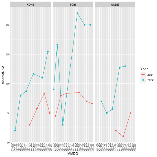
#Next we will visualize the abundance flucutations for Peromyscus leucopus 

# through time:

MNKA_PE<-MNKAbysp %>% filter(taxonID%in%"PELE")



#Create a dataframe with the first date of collection for each bout to use as 

# the date variable when plotting

datedf<-mam_plotNight_nodups %>% 
  select(eventID, collectDate) %>% 
  group_by(eventID) %>%
  summarise(Date = min(collectDate)) %>%
  mutate(Year = substr(Date,1,4), MMDD=substr(Date,6,10))



MNKA_PE<-left_join(MNKA_PE, datedf)



PELEabunplot<-ggplot(data=MNKA_PE, 
                     aes(x=MMDD, y=meanMNKA, color=Year, group=Year)) +
  geom_point() +
  geom_line()+
  facet_wrap(~siteID) +
  theme(axis.text.x =element_text(angle=90))

#group tells ggplot which points to group together when connecting via a line.



PELEabunplot

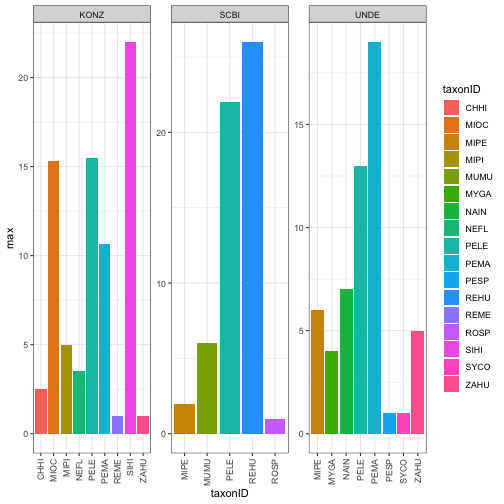
Next we will look at the maximum abundance of the different species recorded at each site over the timespan of the data.

TaxDat<-MNKAbysp %>% 
  group_by(taxonID, siteID) %>% summarise(max=max(meanMNKA))



TaxPlot<-ggplot(TaxDat, aes(x=taxonID, y=max, fill=taxonID)) + 
  geom_bar(stat = "identity")+
  facet_wrap(~siteID, scales = 'free') +
  theme_bw()+
  theme(axis.text.x = element_text(angle=90, vjust=.5, hjust=1))



TaxPlot

4. Visualize Pathogen Prevalence Data at these Sites:

NEON is testing small mammal ear and blood tissue for a variety of tick-borne pathogens. We began with a pilot at a subset of sites in 2020 and expanded to all sites in 2021. Next we will take a look at some of the preliminary results for this new pathogen data product. Interesting extensions can be made to connect these data with the Ticks sampled using drag cloths data product (DP1.10093.001) and Tick pathogen status data product (DP1.10092.001)

#First download the rodent pathogen data

rptdat <- loadByProduct(dpID="DP1.10064.002", 
                         site=c("SCBI", "KONZ", "UNDE"),
                         package="basic", 
                         check.size = FALSE,
                        startdate = "2021-01",
                        enddate = "2022-12")



list2env(rptdat, envir=.GlobalEnv)



#Then check for and deal with any duplicates

rpt_pathres_nodups <- neonOS::removeDups(data=rpt2_pathogentesting,
                             variables=variables_10064,
                             table='rpt2_pathogentesting')

The information about the species from which the samples were taken is found in the small mammal trapping data. Any analyses that will look at species will need to join the trapping data table with the pathogen data table. In Section 2 above we used the joinTableNEON function to join mam_perplotnight data with mam_pertrapnight data. Unfortunately the joinTableNEON function is not an option for the rodent tick-borne pathogen data because of the complexities involved in matching the sample IDs. This is noted in the "Table joining" section of the quick start guide for tick-borne rodent pathogens on the data product landing page.

If you attempt to use that function you will get the error: Error in neonOS::joinTableNEON(mam_pertrapnight, rpt2_pathogentesting) : Tables mam_pertrapnight and rpt2_pathogentesting can't be joined automatically. Consult quick start guide for details about data relationships. Instead we can follow the steps below to join the rodent tick-borne pathogen data with the small mammal trapping data.

#First subset the two dataframes that will be merged to select out a smaller 

# subset of columns to make working with the data easier:

rptdat.merge<-rpt_pathres_nodups %>% 
  select(plotID, collectDate, sampleID, testPathogenName, testResult) %>%
  mutate(Site = substr(plotID,1,4))

mamdat.merge<-mam_trapNight_nodups %>% 
  select(taxonID, bloodSampleID, earSampleID)



#Split the rodent pathogen data by sample types (ear or blood) before joining 

# with the trapping data since there are 2 different columns for sampleID in 

# the mammal trapping data - one for blood samples and one for ear samples.

rptear<-rptdat.merge %>% filter(grepl('.E', sampleID, fixed=T))

rptblood<-rptdat.merge %>% filter(grepl('.B', sampleID, fixed=T))



#Join each sample type with the correct column from the mammal trapping data.

rptear.j<-left_join(rptear, mamdat.merge, by=c("sampleID"="earSampleID"))

rptblood.j<-left_join(rptblood, mamdat.merge, by=c("sampleID"="bloodSampleID"))

rptall<-rbind(rptear.j[,-8], rptblood.j[,-8]) #combine the dataframes after 

# getting rid of the last column whose names don't match and whose data is 

# replaced by the sampleID column

Next we will summarize the prevalence of the different pathogens across sites and species and compare them visually.

#Calculate the prevalence of the different pathogens in the different taxa at 

#each site.

rptprev<-rptall %>%
  group_by(Site, testPathogenName, taxonID) %>% 
  summarise(tot.test=n(), tot.pos = sum(testResult=='Positive')) %>%
  mutate(prevalence = tot.pos/tot.test)



#Barplot of prevalence by site and pathogen name

PathPlot<-ggplot(rptprev, 
                 aes(x=testPathogenName, y=prevalence, fill=testPathogenName)) + 
  geom_bar(stat = "identity")+
  facet_wrap(~Site) +
  theme_bw()+
  theme(axis.text.x = element_text(angle=90, vjust=.5, hjust=1))

PathPlot

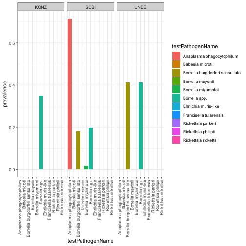
#SCBI seems to have a high prevalence of pathogens - let's look at the 

# prevalence across the species examined for testing:

SCBIpathdat<-rptprev %>% filter(Site %in% 'SCBI')

SCBIPlot<-ggplot(SCBIpathdat, 
                 aes(x=testPathogenName, y=prevalence, fill=testPathogenName)) + 
  geom_bar(stat = "identity")+
  facet_wrap(~taxonID) +
  theme_bw()+
  theme(axis.text.x = element_text(angle=90, vjust=.5, hjust=1))

SCBIPlot

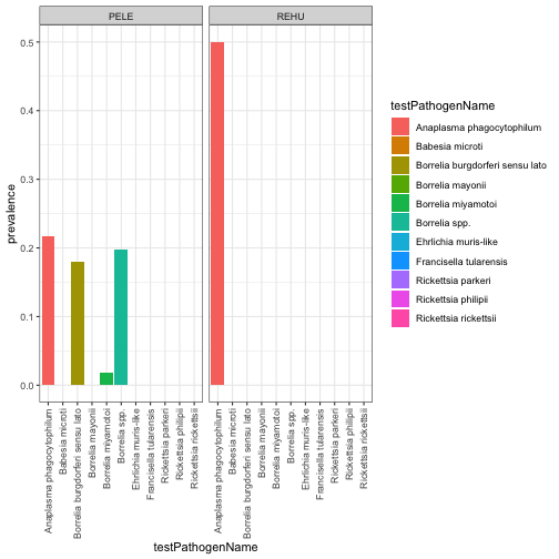
Pathogen distribution and prevalence are governed by a complex array of factors involving hosts, vectors and abiotic variables. It appears from our visualization of these 3 NEON sites that there is a larger diversity of tick-borne pathogens present at SCBI than the other sites co-inciding with a lower diversity of the small mammmal population targeted by our sampling methods. Further analyses could use additional NEON data products such as tick diversity and abundance and/or abiotic conditions related to temperature, humidity and/or soil properties to determine their associations with rodent pathogen diversity and prevalence.