Tutorial
Introduction to the Canopy Nitrogen Data Product - Python
Last Updated: Jun 30, 2026
Canopy Nitrogen (Normalized Difference Nitrogen Index (NDNI)) was one of AOP's original data products, however the first algorithm used (a simple index) was deemed to provide data of insufficient quality for the sensor, scale and site conditions associated with NEON AOP collections. See the November 17, 2020 Data Notification for more details. Over the past years, AOP has been working on implementing an improved algorithm that produces higher quality results. In February 2026, NEON published a new Canopy Nitrogen (%N) data product (DP3.30018.002) for a subset of sites, using models derived from NEON's hyperspectral and foliar chemistry data. We are seeking feedback from the community to review this data product before the model is applied to all of NEON's terrestrial sites. For more details on this data product, refer to the Canopy Nitrogen Quick Start Guide, also found on the Canopy Nitrogen Data Product landing page.
In this tutorial, we demonstrate how to download nitrogen data for a single 1 km 1 km area of the Canopy Nitrogen Data Product over Harvard Forest, and explain the four raster tiles that are associated with this data product. We then show how to use the valid pixel mask to mask out invalid data.
Objectives
After completing this tutorial, you will be able to:
- Download the Canopy Nitrogen rasters
- Understand the 4 raster files that comprise the Canopy Nitrogen data product
- Understand what the needle v. non-needle classification and valid pixel masks mean and how to use them
- Mask the Nitrogen data to include only valid pixels
Things You’ll Need To Complete This Tutorial
To complete this tutorial, you will need:
- Python version 3.9 or higher
- Create a NEON user account
- Generate an API token for downloading data
Install Python Packages
- neonutilities
- rasterio
Let's get started! First import the required Python packages, neonutilities and rasterio as well as some other packages for plotting and interacting with the operating system.
import neonutilities as nu
import os
import numpy as np
import matplotlib.pyplot as plt
import matplotlib.colors as mcolors
import matplotlib.patches as mpatches
import rasterio
from rasterio.plot import show
from rasterio.plot import plotting_extent
import dotenv
As of June 2026, NEON requires an API token for data downloads, to reduce bot scraping and improve user support. Tokens can be generated in NEON data portal user accounts - log in to your account or create one, and go to the API Tokens section. For best practices in storing and using tokens, follow the instructions here. Once you've saved your token, you can load it to a variable called token as follows:
dotenv.load_dotenv()
token = os.environ.get("NEON_TOKEN")
# print(token) # uncomment to display the token; if you haven't set the token properly in the environment, this will print nothing
First let's see what data are available. As of Feb 2026, only a subset of sites have been published, as NEON is seeking input from the user community before producing this model for all NEON terrrestrial sites. See the Data Notification New Data Product: Canopy Nitrogen, Subset of Data Available for Community Review for more details.
nu.list_available_dates(dpid="DP3.30018.002", site="HARV")
PROVISIONAL Available Dates: 2019-08
So far, there is data for HARV in 2019. All of the data is currently Provisional.
Let's first set the download directory (where we will download data) to be in the Downloads folder.
download_dir = os.path.expanduser("~\\Downloads")
Now we can use by_tile_aop to download a single tile for HARV in 2019. We are choosing a tile that includes both forest and part of a lake (the Quabbin Reservoir).
nu.by_tile_aop(dpid="DP3.30018.002", # download the Canopy Nitrogen Product
               site="HARV",
               year=2019,
               easting=723000, # UTM easting
               northing=4708000, # UTM northing
               include_provisional=True, # include provisional data
               savepath=download_dir,
               token=token)
Provisional NEON data are included. To exclude provisional data, use input parameter include_provisional=False.


Continuing will download 5 NEON data files totaling approximately 15.7 MB. Do you want to proceed? (y/n)  y


Downloading 5 NEON data files totaling approximately 15.7 MB

100%|████████████████████████████████████████████████████████████████████████████████████| 5/5 [00:04<00:00,  1.04it/s]
Display the data files that we've downloaded, looking in the download directory. Data is stored in nested paths under the data product id (DP3.30018.002).
nitrogen_dir = os.path.join(download_dir,'DP3.30018.002')
for root, dirs, files in os.walk(nitrogen_dir):
    for file in files:
        print(os.path.join(root.replace(download_dir,'..'),file))
..\DP3.30018.002\citation_DP3.30018.002_PROVISIONAL.txt
..\DP3.30018.002\issueLog_DP3.30018.002.csv
..\DP3.30018.002\neon-aop-provisional-products\2019\FullSite\D01\2019_HARV_6\L3\Spectrometer\Nitrogen\NEON_D01_HARV_DP3_723000_4708000_nitrogen.tif
..\DP3.30018.002\neon-aop-provisional-products\2019\FullSite\D01\2019_HARV_6\L3\Spectrometer\Nitrogen\NEON_D01_HARV_DP3_723000_4708000_nitrogen_classification.tif
..\DP3.30018.002\neon-aop-provisional-products\2019\FullSite\D01\2019_HARV_6\L3\Spectrometer\Nitrogen\NEON_D01_HARV_DP3_723000_4708000_nitrogen_uncertainty.tif
..\DP3.30018.002\neon-aop-provisional-products\2019\FullSite\D01\2019_HARV_6\L3\Spectrometer\Nitrogen\NEON_D01_HARV_DP3_723000_4708000_nitrogen_valid.tif
..\DP3.30018.002\neon-publication\NEON.DOM.SITE.DP3.30018.002\HARV\20190801T000000--20190901T000000\basic\NEON..HARV.DP3.30018.002.readme.20260210T033154Z.txt
The download includes a citation file, issueLog file, readme file, and four geotiff (.tif) files. We encourage you to look through the text files on your own, and please cite NEON data! We will now explore each of the the geotiff files. We can use the rasterio package to read in and display these files.
The four raster files that make up the canopy nitrogen data product are explained briefly below:
-
_nitrogen.tif: mosaicked %N map covering all tiles within each site is available. -
_nitrogen_uncertainty.tif: %N uncertainty map - uncertainty associated with the %N predictions. It is calculated by taking the standard deviation of the %N predictions from each decision tree in the random forest model for each 1 m pixel within the tile. -
_nitrogen_classification.tif: Classification result for needle vs non-needle model, which is a binary map generated using SVM classification, where needle types are coded as 0 and non-needle types as 1 for each 1 m pixel within the tile. The "non-needle" class includes all vegetation types that are not needleleaf, such as broadleaf trees, shrubs, herbaceous cover, and others. Separate random forest regression models have been developed to predict foliar nitrogen values for needle and non-needle vegetation types. -
_nitrogen_valid.tif: Valid pixel mask based on NDVI threshold of 0.2, where values less than 0.2 are set to 0 ("non-valid"). This mask is intended to enable exclusion of non-vegetated areas, such as roads, water bodies, built-up areas, bare rock, and so forth.
The code chunk below shows how to read the four files into variables, which we can then plot.
# read each of the files into the four variables
for root, dirs, files in os.walk(nitrogen_dir):
    for file in files:
        if file.endswith('nitrogen.tif'):
            nitrogen = os.path.join(root,file)
        if file.endswith('nitrogen_uncertainty.tif'):
            nitrogen_uncertainty = os.path.join(root,file)
        if file.endswith('nitrogen_classification.tif'):
            needle_classification = os.path.join(root,file)
        if file.endswith('nitrogen_valid.tif'):
            validity_classification = os.path.join(root,file)
Make a function to display the rasters. This has some custom formatting options and works with both continuous rasters (like the nitrogen and nitrogen uncertainty) as well as the classification rasters (needle / non-needle and valid pixel masks).
# Function to open a raster and plot, including custom formatting options
def plot_neon_raster(file_path, title, cmap, labels=None):
    with rasterio.open(file_path) as src:
        data = src.read(1)
        extent = plotting_extent(src)

        fig, ax = plt.subplots(figsize=(6, 4))

        img = ax.imshow(data, cmap=cmap, extent=extent) # Plot with UTM coordinates
        ax.ticklabel_format(style='plain', axis='both')
        plt.xticks(rotation=45)

        ax.set_title(title)
        ax.set_xlabel('UTM Easting (m)')
        ax.set_ylabel('UTM Northing (m)')

        if labels:
            colors = [cmap(i) for i in range(len(labels))]
            patches = [mpatches.Patch(color=colors[i], label=labels[i])
                       for i in range(len(labels))]
            ax.legend(handles=patches, bbox_to_anchor=(1.05, 1), loc='upper left')
        else:
            fig.colorbar(img, ax=ax)

        plt.tight_layout()
        plt.show()
Plot the four Canopy Nitrogen rasters
Canopy Nitrogen
First let's plot the Canopy Nitrogen (%) raster.
plot_neon_raster(nitrogen, 'Canopy Nitrogen (%)', cmap='viridis');
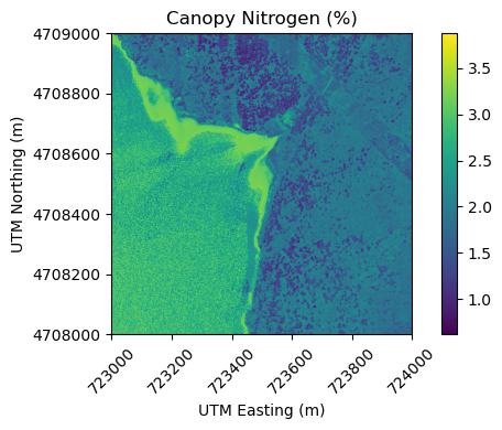
Nitrogen values range from ~1-3.5 percent at the highest. We can also see that there are some values in the reservoir which don't really make sense. Let's look at the uncertainty map next.
Canopy Nitrogen Uncertainty
plot_neon_raster(nitrogen_uncertainty, 'Canopy Nitrogen Uncertainty (%)', cmap='Spectral_r');
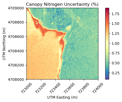
We can see that there are higher uncertainty levels in the reservoir, but over the land the uncertainty is typically < 1%. The Nitrogen values themselves are only around 1-3%, so this is still a fairly high level of uncertainty, relative to the Nitrogen values.
You may also notice a faint vertical line through the middle of the image. This is because the model was created using the surface directional reflectance, and there are some artifacts related to the BRDF effect that are more prominent on the edges of flight lines. In the future, the model will be trained on the bidirectional reflectance (BRDF and topographic corrected) so these artifacts should not appear, or be as prominent.
Next we'll look at the needle / non-needle classification map:
Needle Non-needle Classification
# create a binary blue/yellow color map to display the 2 classes (0 = non-needle, blue & 1 = needle, yellow)
needle_cmap = mcolors.ListedColormap(['#004488', '#DDAA33'])

plot_neon_raster(needle_classification,
                 'Needle / Non-Needle Classification',
                 needle_cmap,
                 labels=['Non-Needle', 'Needle'])
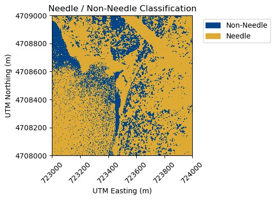
It looks like the forest is a mix of needle and non-needle, which makes sense - there are a lot of deciduous trees in the Northeast, and there are also fields and other vegetation types. There are also classification values in the lake, which don't really make sense. That brings us to the last raster, the validity classification. You can plot that as follows:
Valid Pixel Mask
# create a binary magenta/green color map to display the 2 classes (0 = invalid, magenta & 1 = valid, green)
validity_cmap = mcolors.ListedColormap(['#AA4499', '#117733'])

plot_neon_raster(validity_classification,
                 'Validity Classification (NDVI > 0.2 = valid)',
                 validity_cmap,
                 labels=['Invalid', 'Valid'])
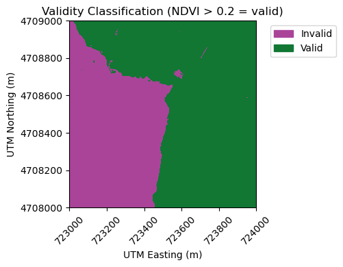
We can see that the water body (Quabbin Reservoir) contains largely non-valid pixels (values are 0). This makes sense - canopy nitrogen does not make sense over water bodies! You may wish to create your own mask, as this just relies on a simple NDVI threshold (anything with NDVI < 0.2 is set to "invalid"). There are some other small areas within the land that are also classified as non-valid. To make a more sophisticated validity mask, you can use a different threshold from the NEON NDVI data product (Vegetation Indices - DP3.30026.001), incorporate other indices, or even use the surface reflectance data directly. We can also see that the areas of higher uncertainty are areas that should not be used anyway.
Mask Nitrogen Data by Valid Pixel Mask
Finally, we can use this valid pixel mask to mask out data in the original Canopy Nitrogen mask.
# Read both rasters (nitrogen and valid pixel map)
with rasterio.open(nitrogen) as src_nitrogen:
    nitrogen_data = src_nitrogen.read(1).astype(float)
    nitrogen_profile = src_nitrogen.profile
    nitrogen_transform = src_nitrogen.transform

with rasterio.open(validity_classification) as src_valid:
    valid_data = src_valid.read(1)

# Mask in one line: set to NaN where validity is 0
nitrogen_masked = np.where(valid_data == 0, np.nan, nitrogen_data)

# Get extent from the raster transform
left, bottom, right, top = rasterio.transform.array_bounds(
    nitrogen_profile['height'], nitrogen_profile['width'], nitrogen_transform)

# plot the masked raster
plt.figure(figsize=(8, 6))
plt.imshow(nitrogen_masked, cmap='viridis', extent=[left, right, bottom, top])
plt.colorbar(label='Canopy Nitrogen (%)')
plt.title('Masked Canopy Nitrogen (%)')
plt.xlabel('UTM Easting (m)')
plt.ylabel('UTM Northing (m)')
plt.ticklabel_format(axis='y', style='plain')
plt.show()
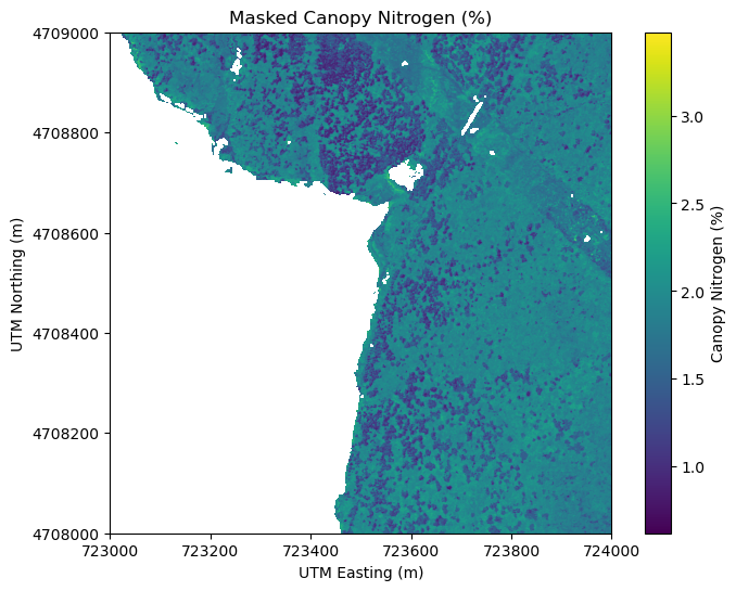
There are some pixels in the lake that were not masked out - these are pixels where the NDVI was > 0.2. You can also see there is a diagonal (NW-SE) strip running across the NE corner of the plot - this could be a clear-cut for powerline or a road. We highly encourage you to look at other imagery, such as the NEON RGB Camera Imagery (DP3.30010.001), the Reflectance RGB Imagery (DP3.30006.001, DP3.30006.002), or even external imagery sources such as Google Earth, or satellite derived land cover classifications to provide more contextual information, and to understand where the nitrogen map makes sense to use. You may also wish to create your own valid pixel mask, but the one provided is intended to give a general sense of where the Nitrogen values can meaningfully be applied.
Recap
In this lesson, you've explored the four raster files that make up the canopy nitrogen data product, and you learned how to apply the valid pixel mask, as well as some caveats to using this validity layer. It is important to pull in additional data sources and to perform your own checks and QA/QC when working with this Nitrogen data product, as with any NEON data. This lesson is intended to show the first step in working with the Canopy Nitrogen data. We hope you explore this data product more on your own!