
Tutorial
Exploring diel carbon flux cycles
Last Updated: Jun 30, 2026
This data tutorial provides an overview of exploring NEON carbon
flux data, using the neonUtilities R package. If you are just starting to work with NEON data it is recommended that you also checkout the more general tutorials, such as the
Download and Explore NEON Data tutorial
or the Introduction to working with NEON eddy flux data. This tutorial builds off the data exploration techniques described in the aforementioned tutorials, and will explore carbon dynamics at two forested ecosystem sites in NEON's Domain 5 - Great Lakes, STEI and TREE. The STEI and TREE sites are only located approximately 1 mile from each other, but experience very different land management practices.
This tutorial assumes general familiarity with eddy-covariance data, and will briefly discuss both turbulent (turb) and storage (stor) fluxes in relation to the net surface atmosphere exchange (nsae). The nsae for CO2 fluxes is often referred to as Net Ecosystem Exchange (NEE).
1. Set up environment and download data
Start by installing and loading packages and setting options. The rhdf5 package is hosted on Bioconductor, requiring BiocManager to be installed to allow rhdf5 to be pulled from the Bioconductor repository. You can skip the installation step if these packages are already installed on your machine, although checking for updates is always wise.
##

## install.packages('BiocManager')

## BiocManager::install('rhdf5')

## install.packages('neonUtilities')

## install.packages('ggplot2')

## install.packages('dplyr')

## install.packages('tidyr')

##

library(neonUtilities)

library(rhdf5)

library(ggplot2)

library(dplyr)

library(tidyr)

##
Now that all the required packages are loaded, let's define all the necessary function arguments to download and stack our flux data using the neonUtilities package's zipsByProduct() and stackEddy() functions. I will define the input arguments as variables to make it easy to modify if I want to explore additional sites or months of data. For this analysis, we will focus on the 2022 growing season at STEI and TREE. Please be aware that the data download size is ~ 1 GB. The code can be modified to shorten or extend this window, but to get a good look at the carbon dynamics at the site it was important to capture most of the growing season.
Inputs to the zipsByProduct() function:
-
dpID: DP4.00200.001, the bundled eddy covariance product -
package: basic (the expanded package has additional quality metrics and advanced footprint matrices that are not relevant to this tutorial) -
site: STEI and TREE -
startate: 2022-04 -
enddate: 2022-09 -
savepath: modify if desired; code below sets to the working directory -
check.size: TRUE if you want to see file size before downloading, otherwise FALSE -
token: NEON API token. Required for data downloads. Tokens can be generated in NEON data portal user accounts - log in to your account or create one, and go to the API Tokens section. For best practices in storing and using tokens, follow the instructions here.
The download may take a while, especially if you're on a slow network. For faster downloads, consider using an API token.
token <- Sys.getenv("NEON_TOKEN")


startDate <- "2022-04"

endDate <- "2022-09"


site <- c("STEI", "TREE")


dirFile <- getwd()


zipsByProduct(dpID="DP4.00200.001", package="basic",
              site=site,
              startdate=startDate,
              enddate=endDate,
              release="RELEASE-2024",
              savepath=dirFile,
              check.size=FALSE,
              token=token)
2. Stacking Level 4 Flux Data
There are five levels of data contained in the eddy flux bundle. For full details, refer to the NEON algorithm document.
In this tutorial we will only be focusing on Level 4 (dp04) flux data products; however, additional data products from Level 0' (dp0p) calibrated raw data to Level 3 (dp03) spatially interpolated vertical profiles used to derive the storage flux are available in the EC bundled HDF5 files. Information can be found on the <a href="NEON algorithm document" target="_blank">NEON Bundled data product - eddy covariance webpage. The Introduction to working with NEON eddy flux data tutorial dives into additional detail regarding the other data product levels, but this tutorial will focus exclusively on flux data.
To extract the dp04 data from the HDF5 files and merge them into a
single table, we'll use the stackEddy() function. We provide the function two input arguments, filepath and level. The filepath will be the file directory (dirFile) used for the data download via zipsByProduct() combined with the filestoStack00200 folder created by the function. To grab just the flux data products level = dp04:
flux <- stackEddy(filepath=paste0(dirFile,
                                  "/filesToStack00200"),
                  level="dp04")
We now have an object called flux. It's a named list containing six
tables: one table for each site's data, plus four metadata tables:
variables and objDesc contain details about the data variables, issue_log
contains records about changes or errors in the data, and citation contains
the BibTeX citation for the downloaded data.
One of the advantages to the HDF5 files is all the metadata and data descriptions can be compiled into file as additional data tables or as attributes. The stackEddy() function stacks this contextual data in the variables and objDesc tables to help you interpret the column headers in the data table (though it's not comprehensive currently).
The terms of interest for our analysis in dp04 the three flux quantities under
fluxCo2:
-
turb: Turbulent flux -
stor: Storage -
nsae: Net surface-atmosphere exchange
Note the variables table contains the units for each field:
flux$variables

##    category   system variable             stat           units
## 1      data  fluxCo2     nsae          timeBgn              NA
## 2      data  fluxCo2     nsae          timeEnd              NA
## 3      data  fluxCo2     nsae             flux umolCo2 m-2 s-1
## 4      data  fluxCo2     stor          timeBgn              NA
## 5      data  fluxCo2     stor          timeEnd              NA
## 6      data  fluxCo2     stor             flux umolCo2 m-2 s-1
## 7      data  fluxCo2     turb          timeBgn              NA
## 8      data  fluxCo2     turb          timeEnd              NA
## 9      data  fluxCo2     turb             flux umolCo2 m-2 s-1
## 10     data  fluxH2o     nsae          timeBgn              NA
## 11     data  fluxH2o     nsae          timeEnd              NA
## 12     data  fluxH2o     nsae             flux           W m-2
## 13     data  fluxH2o     stor          timeBgn              NA
## 14     data  fluxH2o     stor          timeEnd              NA
## 15     data  fluxH2o     stor             flux           W m-2
## 16     data  fluxH2o     turb          timeBgn              NA
## 17     data  fluxH2o     turb          timeEnd              NA
## 18     data  fluxH2o     turb             flux           W m-2
## 19     data fluxMome     turb          timeBgn              NA
## 20     data fluxMome     turb          timeEnd              NA
## 21     data fluxMome     turb         veloFric           m s-1
## 22     data fluxTemp     nsae          timeBgn              NA
## 23     data fluxTemp     nsae          timeEnd              NA
## 24     data fluxTemp     nsae             flux           W m-2
## 25     data fluxTemp     stor          timeBgn              NA
## 26     data fluxTemp     stor          timeEnd              NA
## 27     data fluxTemp     stor             flux           W m-2
## 28     data fluxTemp     turb          timeBgn              NA
## 29     data fluxTemp     turb          timeEnd              NA
## 30     data fluxTemp     turb             flux           W m-2
## 31     data     foot     stat          timeBgn              NA
## 32     data     foot     stat          timeEnd              NA
## 33     data     foot     stat      angZaxsErth             deg
## 34     data     foot     stat         distReso               m
## 35     data     foot     stat    veloYaxsHorSd           m s-1
## 36     data     foot     stat    veloZaxsHorSd           m s-1
## 37     data     foot     stat         veloFric           m s-1
## 38     data     foot     stat distZaxsMeasDisp               m
## 39     data     foot     stat      distZaxsRgh               m
## 40     data     foot     stat         distObkv               m
## 41     data     foot     stat         paraStbl               -
## 42     data     foot     stat      distZaxsAbl               m
## 43     data     foot     stat       distXaxs90               m
## 44     data     foot     stat      distXaxsMax               m
## 45     data     foot     stat       distYaxs90               m
## 46     qfqm  fluxCo2     nsae          timeBgn              NA
## 47     qfqm  fluxCo2     nsae          timeEnd              NA
## 48     qfqm  fluxCo2     nsae           qfFinl              NA
## 49     qfqm  fluxCo2     stor           qfFinl              NA
## 50     qfqm  fluxCo2     stor          timeBgn              NA
## 51     qfqm  fluxCo2     stor          timeEnd              NA
## 52     qfqm  fluxCo2     turb          timeBgn              NA
## 53     qfqm  fluxCo2     turb          timeEnd              NA
## 54     qfqm  fluxCo2     turb           qfFinl              NA
## 55     qfqm  fluxH2o     nsae          timeBgn              NA
## 56     qfqm  fluxH2o     nsae          timeEnd              NA
## 57     qfqm  fluxH2o     nsae           qfFinl              NA
## 58     qfqm  fluxH2o     stor           qfFinl              NA
## 59     qfqm  fluxH2o     stor          timeBgn              NA
## 60     qfqm  fluxH2o     stor          timeEnd              NA
## 61     qfqm  fluxH2o     turb          timeBgn              NA
## 62     qfqm  fluxH2o     turb          timeEnd              NA
## 63     qfqm  fluxH2o     turb           qfFinl              NA
## 64     qfqm fluxMome     turb          timeBgn              NA
## 65     qfqm fluxMome     turb          timeEnd              NA
## 66     qfqm fluxMome     turb           qfFinl              NA
## 67     qfqm fluxTemp     nsae          timeBgn              NA
## 68     qfqm fluxTemp     nsae          timeEnd              NA
## 69     qfqm fluxTemp     nsae           qfFinl              NA
## 70     qfqm fluxTemp     stor           qfFinl              NA
## 71     qfqm fluxTemp     stor          timeBgn              NA
## 72     qfqm fluxTemp     stor          timeEnd              NA
## 73     qfqm fluxTemp     turb          timeBgn              NA
## 74     qfqm fluxTemp     turb          timeEnd              NA
## 75     qfqm fluxTemp     turb           qfFinl              NA
## 76     qfqm     foot     turb          timeBgn              NA
## 77     qfqm     foot     turb          timeEnd              NA
## 78     qfqm     foot     turb           qfFinl              NA
3. Exploring and plotting CO2 flux data
Let's look at some data! First, we will combine the data from the two sites into a single dataframe with an additional factor variable for the site for easier data munging and to create some interesting data exploration visualizations. In this tutorial we utilize the piping operater %>% from the dplyr to allow us to quickly subset, filter, sort, and plot data using just our combined dataframe dfFlux. We start by looking at the turbulent CO2 flux timeseries at TREE with the points colored by qfFinl:
flux$STEI$Site <- "STEI"

flux$TREE$Site <- "TREE"


dfFlux <- rbind.data.frame(flux$STEI, flux$TREE)


dfFlux %>%
    ggplot(aes(timeBgn,
               data.fluxCo2.turb.flux,
               color=factor(qfqm.fluxCo2.turb.qfFinl) )) +
    geom_point() +
    scale_color_brewer(palette="Set2",
                       name="qfFinal") +
    facet_grid(~Site)

## Warning: Removed 1179 rows containing missing values or values outside the scale range (`geom_point()`).
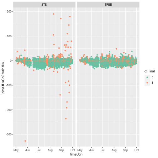
When we plot the data turbulent CO2 flux data, we see a good agreement
between the STEI and TREE sites. We also see some outliers that look to be due to
erroneous data, especially at the STEI site. Fortunately, it looks like final
quality flag (qfFinal = qfFinl) caught the largest outliers, and we can use it to remove
these data from the analysis. Let's first dig into a little background information
about NEON bundled EC quality flags.
Quality flags
The NEON Surface-atmosphere exchange (SAE) data products all come accompanied by
a qfFinal. Information defining the quality flag (qf), quality metric (qm),
and the framework to derive qfFinal are detailed in NEON EC bundled data products algorithm document and
NEON Quality Flags and Quality Metrics for TIS
Data Products algorithm document. Ultimately, for the dp04 flux data
products (e.g. data.fluxCo2.turb.flux), qfFinal of dp01 constituent data
streams derived from plausibility tests (i.e. range test, step test, spike test,
and persistence test) and sensor diagnostic flags, fluxCo2 = rtioMoleDryCo2
and veloZaxsErth (dp01 data outside the scope of tutorial), are propagated and
combined with theoretical eddy-covariance specific quality tests (i.e., stationarity,
integral turbulence characteristics tests) to determine whether the data product
is flagged as valid (qfFinal = 0) or invalid (qfFinal = 1).
Let's summarize our qfqm.fluxCo2.turb.qfFinl to see the total flagged percentage
at our 2 sites.
dfFlux %>%
  group_by(Site) %>%
  summarise(mean(qfqm.fluxCo2.turb.qfFinl))

## # A tibble: 2 × 2
##   Site  `mean(qfqm.fluxCo2.turb.qfFinl)`
##   <chr>                            <dbl>
## 1 STEI                             0.223
## 2 TREE                             0.280
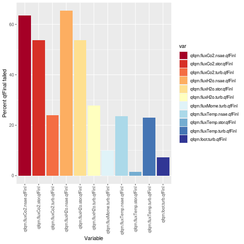
Now, lets plot the qfFinal failed percentage for all our flux data products:
dfFlux %>%
  select(contains("qfqm")) %>%
    pivot_longer(cols = everything(),
                 names_to = "var") %>%
      group_by(var) %>%
        summarise(mean_var = mean(value) * 100) %>%
          ggplot(aes(x = var, y = mean_var,
                     fill = var)) +
          geom_col() +
          guides(x = guide_axis(angle = 90)) +
          labs(x="Variable",
               y="Percent qfFinal failed") +
          scale_fill_brewer(palette="RdYlBu")
Removing data with failed qfFinal
We see that qfqm.fluxCo2.turb.qfFinl is flagged ~ 20-25% over the growing season; however,
the qfqm.fluxCo2.stor.qfFinl and qfqm.fluxCo2.nsae.qfFinl are flagged quite a
bit more due to the complexity of the system and propagation of issues between
sub-components to the overall system (additionally, we currently employ a conservative
quality control for the storage fluxes). Now that we have evaluated the qfFinal
for all the fluxCo2 data streams, lets remove flagged data from our dataframe.
dfFlux %>%
  select(contains("qfqm") &
           contains("fluxCO2")) %>%
  summarise(across(everything(), sum))

##   qfqm.fluxCo2.nsae.qfFinl qfqm.fluxCo2.stor.qfFinl qfqm.fluxCo2.turb.qfFinl
## 1                     9633                     7283                     4423

dfFlux %>%
  select(contains("data") &
           contains("fluxCO2")) %>%
  summarise(across(everything(),
                   function(x)
                     {sum(is.na(x))}))

##   data.fluxCo2.nsae.flux data.fluxCo2.stor.flux data.fluxCo2.turb.flux
## 1                   3195                   2508                   1179

dfFlux$data.fluxCo2.turb.flux[(which(dfFlux$qfqm.fluxCo2.turb.qfFinal==1))] <- NA

dfFlux$data.fluxCo2.stor.flux[(which(dfFlux$qfqm.fluxCo2.stor.qfFinal==1))] <- NA

dfFlux$data.fluxCo2.nsae.flux[(which(dfFlux$qfqm.fluxCo2.nsae.qfFinal==1))] <- NA


dfFlux %>%
  select(contains("qfqm") &
           contains("fluxCO2")) %>%
  summarise(across(everything(), sum))

##   qfqm.fluxCo2.nsae.qfFinl qfqm.fluxCo2.stor.qfFinl qfqm.fluxCo2.turb.qfFinl
## 1                     9633                     7283                     4423

dfFlux %>%
  select(contains("data") &
           contains("fluxCO2")) %>%
  summarise(across(everything(),
                   function(x)
                     {sum(is.na(x))}))

##   data.fluxCo2.nsae.flux data.fluxCo2.stor.flux data.fluxCo2.turb.flux
## 1                   3195                   2508                   1179
We see from the summary of the fluxCo2 qfFinal and data NAs, that the number
of NAs has increased as expected, we have removed all the flagged data from
data.fluxCo2.turb.flux, data.fluxCo2.turb.flux, and
data.fluxCo2.turb.flux. Now we have a clean data set to begin our diel
flux cycle data analysis.
3. Plotting the diel cycle of CO2 fluxes
Let's look at the data in a different way, the diel cycle of carbon and water
vapor are important when evaluating carbon sequestration and ecosystem growth.
We can evaluate the diel cycle by binning the data by hour in the day, this is
relatively straightforward using ggplot and the boxplot function (geom_boxplot()).
dfFlux$hour <- factor(lubridate::hour(dfFlux$timeBgn))


ggplot(dfFlux, aes(x = hour,
                   y = data.fluxCo2.turb.flux,
                   fill = Site)) +
  geom_boxplot() +
  stat_summary(fun = median,
               geom = 'line',
               aes(group = Site,
                   colour = Site))

## Warning: Removed 1179 rows containing non-finite outside the scale range (`stat_boxplot()`).

## Warning: Removed 1179 rows containing non-finite outside the scale range (`stat_summary()`).
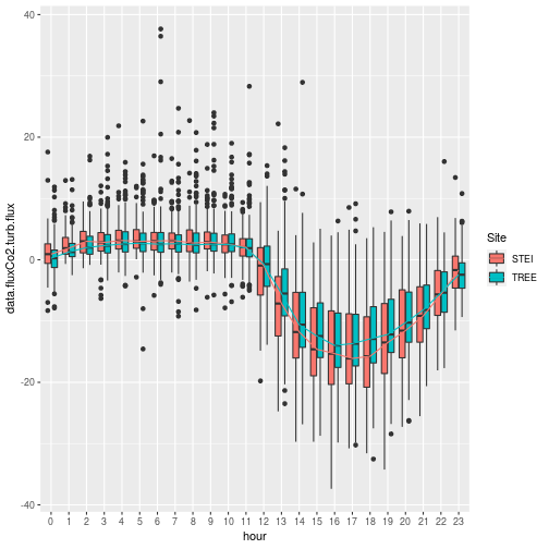
Nice! We get a glimpse of daily carbon dynamics, but something doesn't quite look right.
Note the timing of C uptake; the UTC time zone is clear here, where uptake occurs at times that appear to be during the night. Note that all NEON data use UTC time, aka Greenwich Mean Time. This is true across NEON's instrumented, observational, and airborne measurements. When working with NEON data, it's best to keep everything in UTC as much as possible, otherwise it's very easy to end up with data in mismatched times.
As an illustration, here we will convert to local time for clearer visualization of fluxes in their diel patterns. However, we recommend against doing this in analyses, since it is much more straightforward to keep all data in UTC.
The metadata attributes at the site level in the bundled
EC HDF5 files contains fields for ZoneTime and TimeDiffUtcLt. We can use the
rhdf5 package h5readAttributes() function to grab the metadata. In this
analysis, both the STEI and TREE are in the same timezone. Therefore, we will
only grab metadata from one file and apply to both sites.
fileMeta <- list.files(dirFile,
                       pattern = paste0(".*",
                                        site[1],
                                        ".*.h5"),
                       recursive = TRUE,
                       full.names = TRUE)[1]


siteMeta <- h5readAttributes(fileMeta,
                             name = site[1])


siteMeta

## $DistZaxsCnpy
## [1] 9.5
##
## $DistZaxsDisp
## [1] "6.2"
##
## $DistZaxsGrndOfst
## [1] "0.758"
##
## $DistZaxsLvlMeasTow
## [1] "0.65"  "4.79"  "8.15"  "12.30" "15.66" "22.36"
##
## $DistZaxsTow
## [1] "21.34"
##
## $ElevRefeTow
## [1] "475.7317"
##
## $LatTow
## [1] 45.50895
##
## $LonTow
## [1] -89.58636
##
## $LvlMeasTow
## [1] 6
##
## $`Pf$AngEnuXaxs`
## [1] "0.020097,0.011307,0.012322,0.015949,0.009383,0.007431,0.002004,0.000912,0.002459,-0.002334,0.002954,0.005751,-0.003629,-0.010646,0.001082,-0.001088,0.000915,-0.00618,-0.007461,-0.012817,-0.016043,-0.010921,-0.005637,-0.012574,-0.012343,-0.015775,-0.016883,-0.007593,0.013444,0.02007"
##
## $`Pf$AngEnuYaxs`
## [1] "-0.024191,-0.023851,-0.017583,-0.013608,-0.006831,-0.015542,-0.002694,-0.006488,-0.007339,0.002997,0.013212,0.018439,0.017504,0.017,0.021775,0.017296,0.024619,0.028542,0.020075,0.017117,0.013442,0.018365,0.013516,0.009392,0.009889,-0.003119,-0.000946,0.009277,0.000653,-0.011161"
##
## $`Pf$Ofst`
## [1] "0.016017,0.014884,0.000621,0.008402,0.000912,0.0087,0.007929,0.015406,0.014684,0.011638,0.022359,0.037957,0.03573,0.042482,0.041988,0.02881,0.03758,0.05214,0.034529,0.036575,0.044748,0.041439,0.033977,0.043441,0.053169,0.078641,0.07376,0.0432,0.031761,0.043055"
##
## $TimeDiffUtcLt
## [1] -6
##
## $TimeTube
## [1] 10.1 11.1 10.4 11.3 11.3 12.2
##
## $TypeEco
## [1] "Aspen dominated regenerating forest"
##
## $ZoneTime
## [1] "CST"
##
## $ZoneUtm
## [1] "16N"

dfFlux$timeBgnLst <- dfFlux$timeBgn +
  lubridate::hours(siteMeta$TimeDiffUtcLt)

dfFlux$hourLst <- factor(lubridate::hour(dfFlux$timeBgnLst))


ggplot(dfFlux, aes(x = hourLst,
                   y = data.fluxCo2.turb.flux,
                   fill = Site)) +
  geom_boxplot() +
  stat_summary(fun = median,
               geom = 'line',
               aes(group = Site,
                   colour = Site)) +
  scale_y_continuous(limits = quantile(dfFlux$data.fluxCo2.turb.flux,
                                       c(0.001, 0.999),
                                       na.rm = TRUE))

## Warning: Removed 1213 rows containing non-finite outside the scale range (`stat_boxplot()`).

## Warning: Removed 1213 rows containing non-finite outside the scale range (`stat_summary()`).
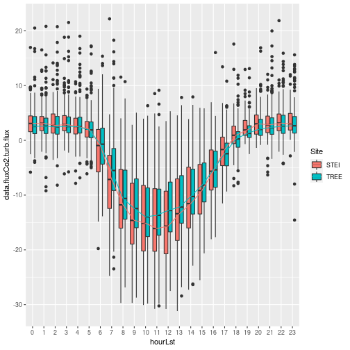
That looks better, now we can clearly see the diel cycle of the turbulent
COsub>2 flux at our STEI and TREE sites with peak carbon uptake around
noon. Carbon uptake generally aligns with peak solar angle and incoming
photosynthetically active radiation (PAR). The boxplot also provides us
information about the variability of the fluxes throughout the day across the
growing season with interquartile range (IQR) represented by the box and the
whiskers indicating the threshold for outliers (black dots) as $ 1.5 x IQR$
subtracted from 1st quantile (Q1) and added to 3rd quantile (Q3):
$$
Q1 - 1.5 * IQR
$$ $$
Q3 + 1.5 * IQR
$$
In the boxplots above the outlier points were greatly reduced after the qfFinal
data removal; however, some outliers remained. To focus our attention on the
bulk of the data, we scaled the y-axis using scale_y_continuous() in conjunction
with the quantile() function to look at 99.8% of the data excluding extreme
outliers that may have remained after our filtering.
We know that the turbulent flux is usually the dominant flux component to NEE,
but the storage flux can be significant at forested sites. Let's have a look at
the storage flux and its impact on the NSAE flux at STEI and TREE:
ggplot(dfFlux, aes(x = hourLst,
                   y = data.fluxCo2.stor.flux,
                   fill = Site)) +
  geom_boxplot() +
  stat_summary(fun = median,
               geom = 'line',
               aes(group = Site,
                   colour = Site)) +
  scale_y_continuous(limits = quantile(dfFlux$data.fluxCo2.stor.flux,
                                       c(0.001, 0.999),
                                       na.rm = TRUE))

## Warning: Removed 2540 rows containing non-finite outside the scale range (`stat_boxplot()`).

## Warning: Removed 2540 rows containing non-finite outside the scale range (`stat_summary()`).
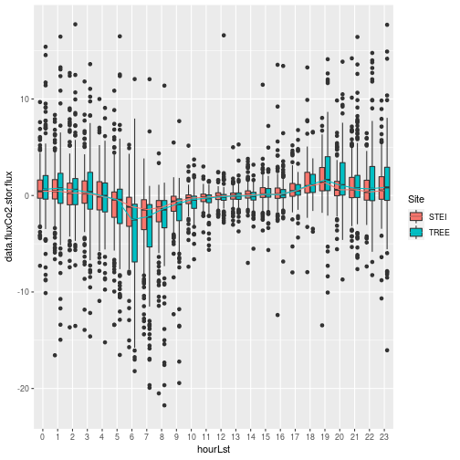
The storage flux as expected is smaller than the turbulent flux, and is dominant during the nighttime hours and evening/morning transition times when turbulence is generally weaker and the trees and understory vegetation aren't photosynthesizing. It's interesting to note the stronger signal at the TREE site. Let's look at how that impacts the overall NSAE flux:
ggplot(dfFlux, aes(x = hourLst,
                   y = data.fluxCo2.nsae.flux,
                   fill = Site)) +
  geom_boxplot() +
  stat_summary(fun = median,
               geom = 'line',
               aes(group = Site,
                   colour = Site)) +
  scale_y_continuous(limits = quantile(dfFlux$data.fluxCo2.nsae.flux,
                                       c(0.001, 0.999),
                                       na.rm = TRUE))

## Warning: Removed 3225 rows containing non-finite outside the scale range (`stat_boxplot()`).

## Warning: Removed 3225 rows containing non-finite outside the scale range (`stat_summary()`).
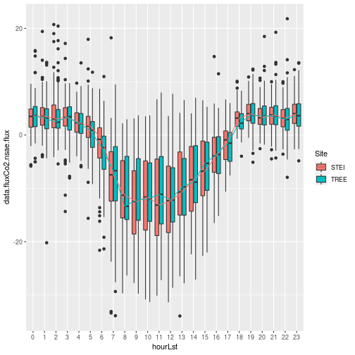
When we look at the NSAE flux we see that the STEI site appears to sequester more carbon, which makes sense considering the STEI site is predominately a young Aspen stand for pulpwood that is growing at a fast rate. It's difficult to get a good total Carbon uptake estimate without performing some more advanced gap-filling and partitioning to better understand the ecosystem carbon dynamics. We can simply look at the relative cumulative flux contributions:
dfFlux %>%
  select(contains("data.fluxCo2") | "Site") %>%
      group_by(Site) %>%
        summarise(across(everything(), mean,
                         na.rm=TRUE))

## # A tibble: 2 × 4
##   Site  data.fluxCo2.nsae.flux data.fluxCo2.stor.flux data.fluxCo2.turb.flux
##   <chr>                  <dbl>                  <dbl>                  <dbl>
## 1 STEI                   -2.44                 0.0486                  -2.47
## 2 TREE                   -1.71                -0.0242                  -1.77
The difference between the two sites is small, but on average the STEI site takes
up more carbon in the turb
CO2 fluxes. This obviously comes with the tradeoff that the trees are
managed for cultivation in the future; whereas, TREE is currently managed as
an educational resource that is likely to be preserved, which may store more
carbon in the longer term.
This analysis is meant to provide a glimpse into NEON flux data products, while focusing primarily on CO2. This workflow can easily be adapted to look at Sensible and Latent heat (H2O) fluxes, or be adapted to evaluate additional NEON sites or years of data.