Tutorial
Working with NEON Site Management Data
Last Updated: May 13, 2026
This tutorial will guide you through accessing, navigating, and working with the NEON data product Site management and event reporting (DP1.10111.001), including how to use code tools in the neonUtilities,geoNEON, and neonSiteMgmtEventData R packages designed specifically for this data product.
If you are new to using NEON data, we recommend first following the Download and Explore tutorial to get familiar with NEON data formats and the neonUtilities package.
Objectives
After completing this activity, you will be able to:
- Download site event data by site or by event type
- Access data related to the spatial extent of an event
- Understand the metadata associated with site events
- Summarize the event data by combinations of site, year, and event type
- Create and export polygons to represent the spatial extent of unique event types
Things You’ll Need To Complete This Tutorial
To complete this tutorial, you will need a version of R (4.0 or higher) and, preferably, RStudio loaded on your computer. This code may work with earlier versions but it hasn't been tested.
Install R Packages
-
neonUtilities:
install.packages("neonUtilities") -
devtools:
install.packages("devtools") -
geoNEON:
devtools::install_github("NEONScience/NEON-geolocation/geoNEON") -
neonSiteMgmtEventData:
devtools::install_github("NEONScience/neonSiteMgmtEventData")
Additional Resources
- Site management and event reporting details page
Site management and event reporting: Background
Events often occur at NEON sites that have an impact on the local ecosystems, but that are not specifically captured in scheduled and planned NEON data collection. These events may be planned or unplanned - for example, controlled burns, wildfires, grazing rotations, and hurricanes. The Site management and event reporting data product is designed to record information about these events. Data are recorded on an ad hoc basis, driven by the occurrence of relevant events.
Event duration and recording
In order to match the publication model for NEON data products and to ensure events are published as quickly as possible, site management and event reporting data are recorded in one-month intervals. This means events longer than one month will have multiple data records for one eventID. The eventID, which includes the site code, original start date, and event type, will remain the same for all records related to the same event. The original start date embedded in the eventID compared to the startDate field for the record indicates if there are related records for previous months. The ongoingEvent field indicates if a record for the next subsequent month is expected.
Date uncertainty is captured in a record’s estimatedOrActualDate field. If the date is estimated additional comments are recorded in the dateRemarks field. The start and end date range includes any date uncertainty.
Set up R environment
First install and load the necessary packages. Skip the install step if packages are already installed, and modify the working directory file path for your computer.
install.packages("neonUtilities")

install.packages("devtools")

devtools::install_github("NEONScience/NEON-geolocation/geoNEON")

devtools::install_github("NEONScience/neonSiteMgmtEventData")

install.packages("ggplot2")

install.packages("dplyr")

install.packages("stringr")

install.packages("tidyr")

install.packages("lubridate")

install.packages("terra")

install.packages("sf")

install.packages("leaflet")

install.packages("magrittr")

install.packages("tidyselect")

install.packages("tibble")


library(neonUtilities)

library(geoNEON)

library(neonSiteMgmtEventData)

library(ggplot2)

library(dplyr)

library(stringr)

library(tidyr)

library(lubridate)

library(terra)

library(sf)

library(leaflet)

library(magrittr)

library(tidyselect)

library(tibble)


setwd("~/data")
Downloading event data: All events at a site
The simplest way to access site event data is to download all the events for a particular site. Let's check out events at Lower Teakettle (TEAK) in California. We'll use include.provisional=T to get events up to the present.
events <- loadByProduct(dpID="DP1.10111.001",
                        site="TEAK",
                        check.size=F,
                        include.provisional=T)
The download includes the usual metadata files associated with NEON data, and two data tables: sim_eventData and sim_locationVisitsAndAttributes.
The sim_locationVisitsAndAttributes table provides a summary of annual visit totals, environmental context, and mitigation actions by location to support estimates of NEON sampling impact and location vulnerability. For TEAK, and all other terrestrial sites, each namedLocation has a record per year for the total unique visits per sampling location. Additional fields describe environmental context (slope, soilOrder, land cover type), document location-specific mitigation measures (such as boardwalks or geoblocks used to minimize trampling), and report the number of sampling events that were cancelled because the location was deemed too vulnerable. Currently, TEAK has no additional mitigation structures, and one sampling bout at TEAK_013 was cancelled in 2025 due to vulnerability. At aquatic sites the total number of visits per site per year is reported, and more specific environmental context fields are not provided.
Let's take a closer look at sim_eventData which documents the external disturbance events.
list2env(events, .GlobalEnv)

## <environment: R_GlobalEnv>

head(sim_eventData)

##                                    uid domainID siteID namedLocation locationID  startDate    endDate ongoingEvent
## 1 2a34be0f-2cb1-4938-8aed-105b6e8b2370      D17   TEAK          TEAK       TEAK 2017-05-01 2017-05-31            Y
## 2 49424b80-bdf1-41ed-9b18-5f34085d5d55      D17   TEAK          TEAK       TEAK 2017-05-31 2017-06-30            Y
## 3 cba1abc5-e6b0-4cd4-b394-ce14f662d295      D17   TEAK          TEAK       TEAK 2017-08-29 2017-09-28            Y
## 4 b28e62bd-76a1-4654-9e1a-8dfd04b611e7      D17   TEAK          TEAK       TEAK 2017-06-30 2017-07-30            Y
## 5 07ae2dab-6622-47a2-9410-0bb4a7a6cff6      D17   TEAK          TEAK       TEAK 2017-07-30 2017-08-29            Y
## 6 07b58f3e-791a-4b13-82f6-36833d41620f      D17   TEAK          TEAK       TEAK 2017-09-28 2017-10-28            Y
##   estimatedOrActualDate dateRemarks               eventID samplingProtocolVersion eventType methodTypeChoice name
## 1                actual        <NA> TEAK.20170501.grazing       NEON.DOC.003282vD   grazing          grazing <NA>
## 2                actual        <NA> TEAK.20170501.grazing       NEON.DOC.003282vD   grazing          grazing <NA>
## 3                actual        <NA> TEAK.20170501.grazing       NEON.DOC.003282vD   grazing          grazing <NA>
## 4                actual        <NA> TEAK.20170501.grazing       NEON.DOC.003282vD   grazing          grazing <NA>
## 5                actual        <NA> TEAK.20170501.grazing       NEON.DOC.003282vD   grazing          grazing <NA>
## 6                actual        <NA> TEAK.20170501.grazing       NEON.DOC.003282vD   grazing          grazing <NA>
##   scientificName otherScientificName fireSeverity biomassRemoval minQuantity maxQuantity quantityUnit reporterType
## 1           <NA>          Bos taurus         <NA>           <NA>           1          25        count    secondary
## 2           <NA>          Bos taurus         <NA>           <NA>           1          25        count    secondary
## 3           <NA>          Bos taurus         <NA>           <NA>           1          25        count    secondary
## 4           <NA>          Bos taurus         <NA>           <NA>           1          25        count    secondary
## 5           <NA>          Bos taurus         <NA>           <NA>           1          25        count    secondary
## 6           <NA>          Bos taurus         <NA>           <NA>           1          25        count    secondary
##                                                                                                                                                                                  remarks
## 1 Low intensity grazing occurs yearlong within the National Forest surrounding TEAK. Quantity of cows are unknown but periodically cows or evidence of cows are spotted within the site.
## 2 Low intensity grazing occurs yearlong within the National Forest surrounding TEAK. Quantity of cows are unknown but periodically cows or evidence of cows are spotted within the site.
## 3 Low intensity grazing occurs yearlong within the National Forest surrounding TEAK. Quantity of cows are unknown but periodically cows or evidence of cows are spotted within the site.
## 4 Low intensity grazing occurs yearlong within the National Forest surrounding TEAK. Quantity of cows are unknown but periodically cows or evidence of cows are spotted within the site.
## 5 Low intensity grazing occurs yearlong within the National Forest surrounding TEAK. Quantity of cows are unknown but periodically cows or evidence of cows are spotted within the site.
## 6 Low intensity grazing occurs yearlong within the National Forest surrounding TEAK. Quantity of cows are unknown but periodically cows or evidence of cows are spotted within the site.
##   recordedBy dataQF  publicationDate      release
## 1       <NA>   <NA> 20251204T234423Z RELEASE-2026
## 2       <NA>   <NA> 20251205T000821Z RELEASE-2026
## 3       <NA>   <NA> 20251205T013836Z RELEASE-2026
## 4       <NA>   <NA> 20251205T014918Z RELEASE-2026
## 5       <NA>   <NA> 20251205T005407Z RELEASE-2026
## 6       <NA>   <NA> 20251205T015325Z RELEASE-2026
Let's first check out the types of events recorded.
sim_eventData |>
  select(eventType, methodTypeChoice) |>
  unique()

##               eventType    methodTypeChoice
## 1               grazing             grazing
## 32  wildlifeDisturbance wildlifeDisturbance
## 59          obstruction         obstruction
## 111                fire       fire-wildfire
TEAK is a managed site, so the events recorded include both acts of nature and active management by the site hosts (grazing).
The neonSiteMgmtEventData package provides a summarizeSIM() function that provides 3 summary tables by site; site and eventType; and site, eventType, and year.
summarizeSIM(df= sim_eventData)

## Sites:  All Sites
## Event Type:  All Event Types

## $summary
##   totalRecords uniqueEvents uniqueEventTypes
## 1          111            4                4
##
## $eventTypeTable
##             eventType TEAK Total
## 1                fire    1     1
## 2             grazing    1     1
## 3         obstruction    1     1
## 4 wildlifeDisturbance    1     1
##
## $yearlyEventTypeTable
##    years           eventType TEAK TotalUniqueEvents
## 1   2017             grazing    1                 1
## 2   2018             grazing    1                 1
## 3   2019             grazing    1                 1
## 4   2019 wildlifeDisturbance    1                 1
## 5   2020             grazing    1                 1
## 6   2021             grazing    1                 1
## 7   2021         obstruction    1                 1
## 8   2022             grazing    1                 1
## 9   2022         obstruction    1                 1
## 10  2023             grazing    1                 1
## 11  2024             grazing    1                 1
## 12  2025                fire    1                 1
## 13  2025             grazing    1                 1
The $summary table sums the number of records in the input dataframe and summarizes the number of individual records, unique events (since a event that is longer than one month will have multiple records), and unique event types.
Next, the $eventTypeTable counts the number of unique eventIDs by eventType and site. The $yearlyEventTypeTable includes grouping by year as well. At TEAK, there are over 100 records but most correspond to a long term grazing event.
There is one wildfire reported. When we look at an event like a fire, we probably want to know exactly where this happened - which NEON sampling areas were burned?
Finding the spatial extent of an event
How to approach the spatial distribution of an event depends on your scientific question. If you're working with data from NEON sampling plots, you might just want to know which plots are affected. You can find that information in the locationID field, which contains either one location or a comma-delimited list of locations for each record. Let's look at the locations associated with the fire in 2025.
burn <- sim_eventData |>
  filter(methodTypeChoice=="fire-wildfire")


burn.locs <- burn |>
  select(locationID) |>
  unlist() |>
  str_split(",") |>
  unlist() |>
  trimws() |>
  unique()


burn.locs

##  [1] "TEAK_001.basePlot.all"      "TEAK_002.basePlot.all"      "TEAK_003.basePlot.all"      "TEAK_006.basePlot.all"
##  [5] "TEAK_007.basePlot.all"      "TEAK_013.basePlot.all"      "TEAK_015.basePlot.all"      "TEAK_017.basePlot.all"
##  [9] "TEAK_018.basePlot.all"      "TEAK_019.basePlot.all"      "TEAK_021.basePlot.all"      "TEAK_024.basePlot.all"
## [13] "TEAK_025.basePlot.all"      "TEAK_001.tickPlot.tck"      "TEAK_002.tickPlot.tck"      "TEAK_006.tickPlot.tck"
## [17] "TEAK_025.tickPlot.tck"      "TEAK_001.mammalGrid.mam"    "TEAK_007.mammalGrid.mam"    "TEAK_025.mammalGrid.mam"
## [21] "TEAK_001.birdGrid.brd"      "TEAK_006.birdGrid.brd"      "TEAK_007.birdGrid.brd"      "TEAK_031.birdGrid.brd"
## [25] "TEAK_038.mosquitoPoint.mos" "TEAK_039.mosquitoPoint.mos" "TEAK_041.mosquitoPoint.mos"
Now we have a list of NEON named locations. We can see if the plot(s) we are working with are on the list, and proceed accordingly.
But what if we're interested in a broader picture, and we want to get a sense of the overall burned area?
Below, we'll find spatial data associated with point locations of disturbance events and create a polygon to export as an sf object, shapefile, or kml for Google Earth.
Caveats about locations:
NEON field staff do their best to record the extent of a disturbance in the list of locations. In the case of planned disturbances, such as controlled burns and release of animals for grazing, the site host may be able to provide a very clear assessment of the locations affected. But for unplanned events such as wildfires or bark beetle outbreaks, these data depend on staff being in the right place at the right time to observe the disturbance. At some NEON sites, sampling plots are very far apart, and if staff are on-site for a particular protocol and only sampling a subset of plots, they may not know the impact of disturbance on other plots.
These limitations primarily affect terrestrial sites. At aquatic sites, sampling locations are clustered in a fairly small area, and staff can more easily assess the extent of a disturbance. In addition, due to the close proximity of sampling, most significant events affect the entire aquatic sampling area.
Finally, we have limited information available about the impact of events outside of NEON sampling locations. A patchy event like a small wildfire may affect locations very unevenly. NEON AOP flights typically cover a 10 x 10 km box that includes the sampling locations, but also includes large areas where NEON does not sample. If you are analyzing a disturbance using remote sensing data, the locations identified in this data product may only be a small subset of the disturbed area within the AOP flight box.
Downloading event data by event type
In many cases, you may be interested in a particular type of disturbance across sites, rather than in various disturbances within a site. Above, we found a report of a fire at TEAK, which is in the mountains in California. In recent years, the western US has experienced a large number of fires, and many of the individual fires have been unusually large. Let's look for all the fires that have affected NEON sites in California. We can do this using the neonUtilities::byEventSIM() function:
fires <- byEventSIM(eventType="fire",
                    site=c("SJER","SOAP","BIGC","TEAK","TECR"),
                    include.provisional=T)
The set of files returned by this function is the same as loadByProduct(), but the data in sim_eventData are filtered down to only the events where the eventType is "fire".
Let's start by looking at the siteID, startDate, endDate, and methodTypeChoice fields to see which sites and years experienced fires.
fires$sim_eventData |>
  select(siteID, startDate, endDate, methodTypeChoice)

##    siteID  startDate    endDate    methodTypeChoice
## 1    BIGC 2020-09-04 2020-10-04       fire-wildfire
## 2    BIGC 2020-10-04 2020-11-03       fire-wildfire
## 3    BIGC 2020-11-03 2020-12-03       fire-wildfire
## 4    BIGC 2020-12-03 2020-12-24       fire-wildfire
## 5    BIGC 2021-06-29 2021-07-08       fire-wildfire
## 6    SJER 2021-11-01 2021-11-16       fire-wildfire
## 7    SOAP 2020-02-24 2020-03-09 fire-controlledBurn
## 8    SOAP 2020-09-04 2020-10-04       fire-wildfire
## 9    SOAP 2020-10-04 2020-11-03       fire-wildfire
## 10   SOAP 2020-11-03 2020-12-03       fire-wildfire
## 11   SOAP 2020-12-03 2020-12-24       fire-wildfire
## 12   SOAP 2021-06-29 2021-07-08       fire-wildfire
## 13   TEAK 2025-08-24 2025-09-22       fire-wildfire
## 14   TECR 2025-08-30 2025-09-29       fire-wildfire
We can also look at summary table by year using neonSiteMgmtEventData::summarizeSIM()
fireSummary <- summarizeSIM(df= fires$sim_eventData)

## Sites:  All Sites
## Event Type:  All Event Types

fireSummary$yearlyEventTypeTable

##   years eventType BIGC SJER SOAP TEAK TECR TotalUniqueEvents
## 1  2020      fire    1    0    3    0    0                 4
## 2  2021      fire    1    1    1    0    0                 3
## 3  2025      fire    0    0    0    1    1                 2
We know 2020 was a terrible year for wildfires in the western US, and unsurprisingly many of the records here are from 2020. But there is also one controlled burn from early 2020, as well as fires in 2021 and 2025.
Let's say we want to use these locations to find NEON remote sensing data for the affected regions, and see where the burned locations appear in the images. We can use the geoNEON package to get the coordinates of the locations listed in the event data.
fire.loc <- getLocTOS(fires$sim_eventData,
                      "sim_eventData")
The getLocTOS() function works slightly differently for site management data than other NEON data products. Because the locations in event data can be a list, the table of geographic information is stored as a nested data frame in the locationID field. To look at the geographic data for just one event, we can extract the nested table. Let's look at the location of the controlled burn in early 2020:
fire.loc$locationID[7]
## [[1]]
## namedLocation locationDescription domainID siteID locationCurrent locationStartDate
## 1 SOAP_003.tickPlot.tck Plot "SOAP_003" at site "SOAP" D17 SOAP TRUE 2010-01-01T00:00:00Z
## 2 SOAP_007.basePlot.all Plot "SOAP_007" at site "SOAP" D17 SOAP TRUE 2010-01-01T00:00:00Z
## 3 SOAP_016.basePlot.all Plot "SOAP_016" at site "SOAP" D17 SOAP TRUE 2010-01-01T00:00:00Z
## 4 SOAP_017.basePlot.all Plot "SOAP_017" at site "SOAP" D17 SOAP TRUE 2010-01-01T00:00:00Z
## 5 SOAP_018.basePlot.all Plot "SOAP_018" at site "SOAP" D17 SOAP TRUE 2010-01-01T00:00:00Z
## 6 SOAP_019.basePlot.all Plot "SOAP_019" at site "SOAP" D17 SOAP TRUE 2010-01-01T00:00:00Z
## 7 SOAP_036.mosquitoPoint.mos Plot "SOAP_036" at site "SOAP" D17 SOAP TRUE 2010-01-01T00:00:00Z
## 8 SOAP_039.mosquitoPoint.mos Plot "SOAP_039" at site "SOAP" D17 SOAP TRUE 2010-01-01T00:00:00Z
## 9 SOAP_041.mosquitoPoint.mos Plot "SOAP_041" at site "SOAP" D17 SOAP TRUE 2010-01-01T00:00:00Z
## decimalLatitude decimalLongitude elevation easting northing utmZone namedLocationCoordUncertainty
## 1 37.03299 -119.249666 1135.91 299905.83167 4100898.65583 11N 0.14
## 2 37.028597 -119.249997 1194.27 299864.85317 4100411.91612 11N 0.1
## 3 37.028524 -119.253018 1205.89 299595.90776 4100410.1795 11N 0.1
## 4 37.030901 -119.242317 1142.85 300554.1072 4100651.4236 11N 0.11
## 5 37.028985 -119.243605 1204.66 300434.51203 4100441.53199 11N 0.1
## 6 37.030844 -119.245692 1182.84 300253.72138 4100652.18439 11N 0.1
## 7 37.034408 -119.243066 1052.06 300496.65662 4101042.12275 11N 10.47
## 8 37.031342 -119.262184 1198.13 298787.92115 4100742.2176 11N 20.49
## 9 37.031894 -119.251043 1156.97 299780.45941 4100779.94541 11N 20.1
## namedLocationElevUncertainty coordinateSource country county geodeticDatum stateProvince utmHemisphere utmZoneNumber
## 1 0.14 GeoXH 6000 unitedStates Fresno WGS84 CA N 11
## 2 0.1 GeoXH 6000 unitedStates Fresno WGS84 CA N 11
## 3 0.1 Geo 7X (H-Star) unitedStates Fresno WGS84 CA N 11
## 4 0.11 Geo 7X (H-Star) unitedStates Fresno WGS84 CA N 11
## 5 0.1 Geo 7X (H-Star) unitedStates Fresno WGS84 CA N 11
## 6 0.1 Geo 7X (H-Star) unitedStates Fresno WGS84 CA N 11
## 7 1.01 Geo 7X (H-Star) unitedStates Fresno WGS84 CA N 11
## 8 0.64 Geo 7X (H-Star) unitedStates Fresno WGS84 CA N 11
## 9 0.1 Geo 7X (H-Star) unitedStates Fresno WGS84 CA N 11
## alphaOrientation betaOrientation gammaOrientation xOffset yOffset zOffset locationEndDate filteredPositions plotHdop
## 1 0 0 0 0 0 0 <NA> 356 3.5
## 2 0 0 0 0 0 0 <NA> 439 1
## 3 0 0 0 0 0 0 <NA> 392 1.1
## 4 0 0 0 0 0 0 <NA> 411 1.1
## 5 0 0 0 0 0 0 <NA> 461 1.1
## 6 0 0 0 0 0 0 <NA> 457 1.4
## 7 0 0 0 0 0 0 <NA> 700 2.7
## 8 0 0 0 0 0 0 <NA> 707 5.3
## 9 0 0 0 0 0 0 <NA> 700 3.6
## maximumElevation minimumElevation plotPdop slopeAspect slopeGradient nlcdClass plotDimensions plotID plotSize
## 1 1138.16 1130.86 6.6 57 9 evergreenForest 40m x 40m SOAP_003 1600
## 2 1202.44 1188.53 2.1 130 8.53 evergreenForest 40m x 40m SOAP_007 1600
## 3 1210.62 1195.51 2.7 342.5 18.83 evergreenForest 40m x 40m SOAP_016 1600
## 4 1153.86 1126.8 2.8 45 24.23 evergreenForest 40m x 40m SOAP_017 1600
## 5 1207.18 1195.92 1.9 228.8 14.09 evergreenForest 40m x 40m SOAP_018 1600
## 6 1188.82 1178.83 2.7 45 7.13 evergreenForest 40m x 40m SOAP_019 1600
## 7 1052.06 1052.06 6.6 290 15 evergreenForest 0m SOAP_036 0
## 8 1198.13 1198.13 6.5 115 14 evergreenForest 0m SOAP_039 0
## 9 1156.97 1156.97 5.4 301 6 shrubScrub 0m SOAP_041 0
## subtype plotType referencePointPosition soilTypeOrder siteType siteTimezone stateAbbreviation subtypeSpecification
## 1 tickPlot distributed 41 Alfisols <NA> <NA> <NA> <NA>
## 2 basePlot distributed 41 Alfisols <NA> <NA> <NA> <NA>
## 3 basePlot distributed 41 Alfisols <NA> <NA> <NA> <NA>
## 4 basePlot distributed 41 Alfisols <NA> <NA> <NA> <NA>
## 5 basePlot distributed 41 Alfisols <NA> <NA> <NA> <NA>
## 6 basePlot distributed 41 Alfisols <NA> <NA> <NA> <NA>
## 7 mosquitoPoint distributed 41 Alfisols <NA> <NA> <NA> <NA>
## 8 mosquitoPoint distributed 41 Alfisols <NA> <NA> <NA> <NA>
## 9 mosquitoPoint distributed 41 Alfisols <NA> <NA> <NA> <NA>
## type description locationPointID locationType locationParent locationParentUrl referenceLocation.locationName
## 1 NA NA NA NA NA NA NA
## 2 NA NA NA NA NA NA NA
## 3 NA NA NA NA NA NA NA
## 4 NA NA NA NA NA NA NA
## 5 NA NA NA NA NA NA NA
## 6 NA NA NA NA NA NA NA
## 7 NA NA NA NA NA NA NA
## 8 NA NA NA NA NA NA NA
## 9 NA NA NA NA NA NA NA
## referenceLocation.locationDecimalLatitude referenceLocation.locationDecimalLongitude referenceLocation.locationElevation
## 1 NA NA NA
## 2 NA NA NA
## 3 NA NA NA
## 4 NA NA NA
## 5 NA NA NA
## 6 NA NA NA
## 7 NA NA NA
## 8 NA NA NA
## 9 NA NA NA
## referenceLocation.locationUtmEasting referenceLocation.locationUtmNorthing
## 1 NA NA
## 2 NA NA
## 3 NA NA
## 4 NA NA
## 5 NA NA
## 6 NA NA
## 7 NA NA
## 8 NA NA
## 9 NA NA
We have coordinates and metadata for each location noted as affected by the controlled burn.
Let's focus on SOAP, and get the locations for all of the areas burned at SOAP in 2020. The unnest() function in the tidyr package can pull out the nested tables and merge them with the data table. This will replicate each row in the original table for every row in the corresponding location table.
fire.SOAP <- fire.loc |>
  filter(siteID=="SOAP" & endDate<"2021-01-01") |>
  unnest(cols="locationID", names_sep="_")
We can now use the easting and northing coordinates to download tiles of AOP data for these locations. SOAP was flown in 2019 and 2021, so we can download before-and-after data. Let's look at NDVI data and see if there is a change in vegetation greenness after the fires.
byTileAOP("DP3.30026.001", site="SOAP", year=2019,
          easting=fire.SOAP$locationID_easting,
          northing=fire.SOAP$locationID_northing,
          buffer=10, check.size=F, savepath=getwd())


byTileAOP("DP3.30026.001", site="SOAP", year=2021,
          easting=fire.SOAP$locationID_easting,
          northing=fire.SOAP$locationID_northing,
          buffer=10, check.size=F, savepath=getwd())
Vegetation indices are downloaded as zip files, so first we need to unzip them.
zippaths <- list.files(getwd(), pattern=".zip",
                        full.names=T, recursive=T)


for(i in 1:length(zippaths)) {
  unzip(zippaths[i], exdir=dirname(zippaths[i]))
}

## Warning in unzip(zippaths[i], exdir = dirname(zippaths[i])): error 1 in extracting from zip file

## Warning in unzip(zippaths[i], exdir = dirname(zippaths[i])): error 1 in extracting from zip file
We'll start with the pre-fire 2019 data. We've downloaded 8 tiles, so we need to read them in and merge them into a single raster.
tiles2019 <- list.files(getwd(), pattern="NDVI.tif",
                        full.names=T, recursive=T)

tiles2019 <- grep("2019", tiles2019, value=T)


ndvi2019 <- rast(tiles2019[1])

for(i in 2:length(tiles2019)) {
  ndvii <- rast(tiles2019[i])
  ndvi2019 <- merge(ndvi2019, ndvii)
}
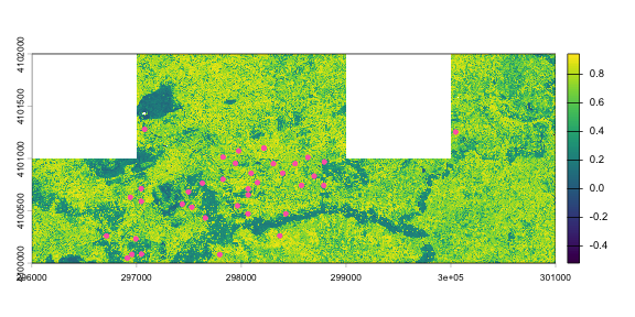
And now plot the canopy height model data, with the burned locations marked as dots. Let's plot the wildfire first, and then add the controlled burn locations.
plot(ndvi2019)


wf.SOAP <- fire.SOAP |>
  filter(methodTypeChoice=="fire-wildfire")

points(wf.SOAP$locationID_easting,
       wf.SOAP$locationID_northing,
       pch=20, col="hotpink")
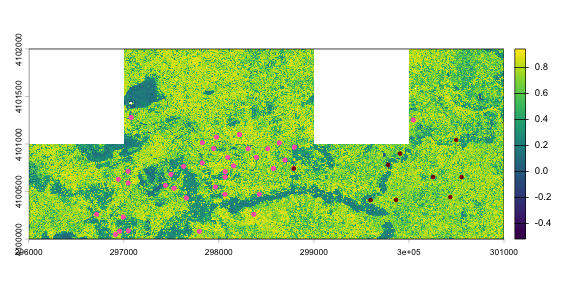
plot(ndvi2019)


points(wf.SOAP$locationID_easting,
       wf.SOAP$locationID_northing,
       pch=20, col="hotpink")


cb.SOAP <- fire.SOAP |>
  filter(methodTypeChoice=="fire-controlledBurn")

points(cb.SOAP$locationID_easting,
       cb.SOAP$locationID_northing,
       pch=20, col="darkred")
We can utilize the neonSiteMgmtEventData package's createSIMPolygon() function to create a polygon around the point locations for each event. The input to createSIMPolygon() is the output of geoNEON::getLocTOS().
# wildfire polygons

wf.SOAP.df <- fire.loc |>
  filter(siteID=="SOAP" & endDate<"2021-01-01" &
           eventType == "fire" &
           methodTypeChoice=="fire-wildfire")


wf.SOAP.polygon <- createSIMPolygon(df= wf.SOAP.df)


# transform the polygon from WGS84 (standard output) to utm zone 11N

# to match AOP tiles.

# coordinate reference system (crs) EPSG values can be searched for

# on https://spatialreference.org/ref/epsg/

wf.SOAP.polygon.utm <- st_transform(wf.SOAP.polygon$sfObjects[[1]],
                                    crs = 32611)


# controlled burn polygons

cb.SOAP.df <- fire.loc |>
  filter(siteID=="SOAP" & endDate<"2021-01-01" &
           eventType == "fire" &
           methodTypeChoice=="fire-controlledBurn")


cb.SOAP.polygon <- createSIMPolygon(df= cb.SOAP.df)


# transform the polygon from WGS84 (standard output) to utm zone 11N

# to match AOP tiles.

# coordinate reference system (crs) EPSG values can be searched for

# on https://spatialreference.org/ref/epsg/

cb.SOAP.polygon.utm <- st_transform(cb.SOAP.polygon$sfObjects[[1]],
                                    crs = 32611)


plot(ndvi2019)


points(wf.SOAP$locationID_easting,
       wf.SOAP$locationID_northing,
       pch=20, col="hotpink")


cb.SOAP <- fire.SOAP |>
  filter(methodTypeChoice=="fire-controlledBurn")

points(cb.SOAP$locationID_easting,
       cb.SOAP$locationID_northing,
       pch=20, col="darkred")


plot(sf::st_geometry(wf.SOAP.polygon.utm),
       border = "hotpink",
       lwd = 2.5,
       add = TRUE)


plot(sf::st_geometry(cb.SOAP.polygon.utm),
       border = "darkred",
       lwd = 2.5,
       add = TRUE)
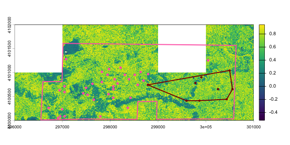
We can see the wildfire polygon (light pink) include the entire site boundary since the site code "SOAP" was one of listed locationIDs.
The controlled burn polygon (dark red) was created as the smallest convex polygon around the listed locationID points.
The polygons provide our best estimate for the actual extent of the event across the site.
And now let's look at the same locations in 2021.
tiles2021 <- list.files(getwd(), pattern="NDVI.tif",
                        full.names=T, recursive=T)

tiles2021 <- grep("2021", tiles2021, value=T)


ndvi2021 <- rast(tiles2021[1])

for(i in 2:length(tiles2021)) {
  ndvii <- rast(tiles2021[i])
  ndvi2021 <- merge(ndvi2021, ndvii)
}


plot(ndvi2021)


points(wf.SOAP$locationID_easting,
       wf.SOAP$locationID_northing,
       pch=20, col="hotpink")


points(cb.SOAP$locationID_easting,
       cb.SOAP$locationID_northing,
       pch=20, col="darkred")


plot(sf::st_geometry(wf.SOAP.polygon.utm),
       border = "hotpink",
       lwd = 2.5,
       add = TRUE)


plot(sf::st_geometry(cb.SOAP.polygon.utm),
       border = "darkred",
       lwd = 2.5,
       add = TRUE)
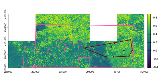
We can see a large region where NDVI is substantially lower in 2021 than 2019, matching the region where the wildfire was reported. Note there is some ambiguity in the region where the controlled burn was reported - it's inside the overall wildfire polygon, but those specific points weren't reported as burned by the wildfire. They are included because the site as a whole was reported.
In addition, we only downloaded the 8 NDVI tiles overlapping the sampling locations that were reported as affected by the fire; the entire AOP footprint is much larger than this. As noted above, NEON field staff report events at locations they visit, but in this case the fire was much larger than the NEON sampling region. The implications of this depend on your analytical goals. If you are studying fire at a regional level, you may focus primarily on the AOP data, whereas if you are primarily interested in plant community responses, you may want to focus on plant presence and percent cover plots, and the status of those specific plots.
If helpful for further analysis, we can export the polygons into a shapefile or kml using sim_locationVisitsAndAttributes::writeExportFile().
# export the wildfire polygons as kmls

writeExportFile(sfList = wf.SOAP.polygon$sfObjects,
                outDir = getwd(),
                outType = "kml")


# export the controlled burns polygons as shapefiles

writeExportFile(sfList = cb.SOAP.polygon$sfObjects,
                outDir = getwd(),
                outType = "shapefile")

## Warning in abbreviate_shapefile_names(obj): Field names abbreviated for ESRI Shapefile driver
For more information and examples using the createSIMPolygon() function please see the vignette associated with the package.
devtools::install_github('NEONScience/neonSiteMgmtEventData',
                force = TRUE, build_vignettes = TRUE)
browseVignettes("neonSiteMgmtEventData")