Plotting and Clustering Megapit Soils Data

This tutorial will show you how to download NEON Megapit soils data, plot soil profiles by texture and chemical properties, and cluster the different megapit profiles according to their similarity across multiple dimensions.

Set up code environment

Before we get the data, we need to install (if not already done) and load the R packages needed for data load and analysis.

As of June 2026, NEON requires an API token for data downloads, to reduce bot scraping and improve user support. Tokens can be generated in NEON data portal user accounts - log in to your account or create one, and go to the API Tokens section. For best practices in storing and using tokens, follow the instructions here.

Install packages:

install.packages("neonUtilities")

install.packages("neonOS")

install.packages("aqp")

install.packages("cluster")

install.packages("sharpshootR")

install.packages("dplyr")

install.packages("Ternary")

Load packages and API token.

# Load required packages

library(neonUtilities)

library(neonOS)

library(aqp)

library(cluster)

library(sharpshootR)

library(dplyr)

library(Ternary)



token <- Sys.getenv("NEON_TOKEN")

Download megapit data

Documentation about the Megapit physical and chemical properties data product can be found here:

• Soil physical and chemical properties, Megapit DP1.00096.001

If you are unfamiliar with neonUtilities and NEON data download workflows, we recommend starting with the Download and Explore NEON Data tutorial.

In this exercise, we want all available data, so we won't subset by site or date range.

MP <- loadByProduct(dpID="DP1.00096.001", 
                    check.size = F,
                    token=token)



list2env(MP, .GlobalEnv)

Join tables and convert to custom soil profile format

We'll join the horizon data to the physical and chemical characteristics data in order to see a depth profile of biogeochemical characteristics. The neonOS package contains the joinTableNEON() function, which uses metadata from the data product's Quick Start Guide to join tables.

S <- joinTableNEON(mgp_perhorizon,
                   mgp_perbiogeosample)



S <- arrange(S, siteID, horizonTopDepth)

There are two more things that we need to do before converting this data frame into a SoilProfileCollection object. First, we will make a new siteLabel column to use when plotting several pedons at once.

## combine 'domainID' and 'siteID' into a new label variable

S$siteLabel <- sprintf("%s-%s", S$domainID, S$siteID)

Second, we will translate the soil physical properties (sand, silt, clay percentages) into an RGB color scheme that we can use for plotting later. These steps are much easier to do now while the data are in a simple data frame.

# duplicate physical property variables

S$r <- S$sandTotal # Sand is Red 'r'

S$g <- S$siltTotal # Silt is Green 'g'

S$b <- S$clayTotal # Clay is Blue 'b'



# set NA values to 100 (white)

S$r[is.na(S$r)] <- 100

S$g[is.na(S$g)] <- 100

S$b[is.na(S$b)] <- 100



# normalize values to 1 and convert to vector of colors using 'rgb()' function

S$textureColor <- rgb(red=S$r/100, 
                      green=S$g/100, 
                      blue=S$b/100, 
                      alpha=1, 
                      maxColorValue = 1)

We now have a data frame of biogeochemical data, organized by site and horizon. We can convert this to a SoilProfileCollection object using the aqp package.

depths(S) <- siteLabel ~ horizonTopDepth + horizonBottomDepth

We then move the site-level metadata to the @site attributes of S, our AQP object. This makes our S object easy to subset to look at a particular site. (Thanks to Dylan Beaudette of the USDA-NRCS for the helpful tips on how to best use this package!)

site(S) <- ~ siteID + nrcsDescriptionID

Plot simple soil profiles

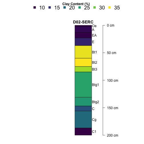
Using the plotting functions in the aqp package, let's start exploring some depth profiles. We'll start with a single site, the Smithsonian Environmental Research Center (SERC), and plot clay content by depth.

# set plot margins

par(mar=c(1,0,3,15), mfrow=c(1,1), xpd=NA)



# Plot SERC clay profile

plotSPC(subset(S, siteID=="SERC"), 
        name='horizonName.x', label='siteLabel', 
        color='clayTotal', col.label='Clay Content (%)',
        col.palette=viridis::viridis(10), 
        cex.names=1, width = 0.1, 
        depth.axis = list(style="traditional",
                          line=6,
                          cex=1), 
        col.legend.cex = 1.5, n.legend=6, 
        x.idx.offset = 0, n=.88)

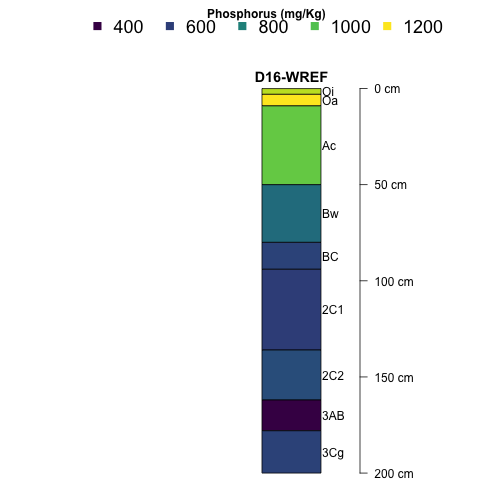
Now let's take a look at phosphorus at Wind River Experimental Forest (WREF).

par(mar=c(1,0,3,15), mfrow=c(1,1), xpd=NA)



plotSPC(subset(S, siteID=="WREF"),  
        name='horizonName.x', label='siteLabel', 
        color='pMjelm', 
        col.label='Phosphorus (mg/Kg)',
        col.palette=viridis::viridis(10), 
        cex.names=1, width = 0.1, 
        depth.axis = list(style="traditional",
                          line=6,
                          cex=1), 
        col.legend.cex = 1.5, n.legend=4, 
        x.idx.offset = 0, n=.88)

Plotting multiple sites

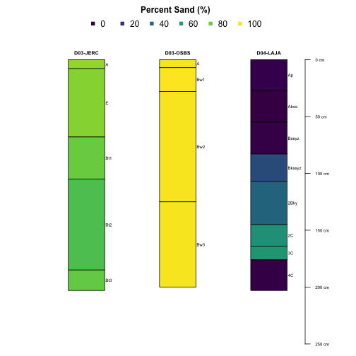
We can pass the plotting function multiple sites in order to compare pedons directly. We'll choose three very different sites with very different soils: Guanica (GUAN), a subtropical dry forest in Puerto Rico, Jornada (JORN), a desert in New Mexico, and Wind River (WREF), a temperate rainforest in Washington State.

par(mar=c(0,2,3,2.5), mfrow=c(1,1), xpd=NA)



plotSPC(subset(S, siteID %in% c('WREF', 'JORN', 'GUAN')),
        name='horizonName.x', label='siteLabel', 
        color='sandTotal', 
        col.label='Percent Sand (%)',
        col.palette=viridis::viridis(10),
        n.legend = 5)

Multivariate plotting

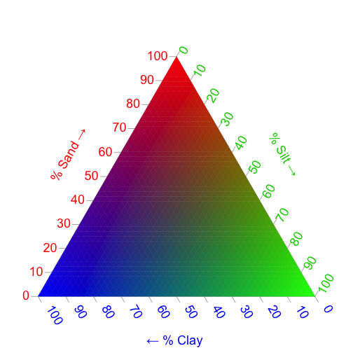
When analyzing soils data, we are often interested in more than one variable at a time. A classic example is texture, which in its simplest terms, is described in terms of percent Sand, Silt, and Clay. In order to plot these three variables together, we can describe each percentage as a color on the color wheel. Remember, in the section above, we assigned the color Red to Sand, Green to Silt, and Blue to Clay. We can plot these colors on the familiar three-axis plot that is often used to describe soil texture to serve as our color legend. To do this, we will use the Ternary package:

par(mfrow=c(1, 1), mar=rep(.3, 4))



TernaryPlot(alab="% Sand \u2192", blab="% Silt \u2192", clab="\u2190 % Clay ",
            lab.col=c('red', 'green3', 'blue'),
            point='up', lab.cex=1.5, grid.minor.lines=1, axis.cex=1.5,
            grid.lty='solid', col=rgb(0.9, 0.9, 0.9), grid.col='white', 
            axis.col=rgb(0.6, 0.6, 0.6), ticks.col=rgb(0.6, 0.6, 0.6),
            padding=0.08)



cols <- TernaryPointValues(rgb)



ColourTernary(cols, spectrum = NULL, resolution=45)

Now, we can plot the soil texture of pedons as a color scheme:

par(mar=c(0,2,3,2.5), mfrow=c(1,1), xpd=NA)



plotSPC(subset(S, siteID %in% c('WREF', 'JORN', 'GUAN')),
        name='horizonName.x', label='siteLabel', 
        color='textureColor')

Multivariate clustering

We have 47 Megapit samples across the NEON observatory, spanning a wide range of soil types, textures, and chemical profiles. While it may be helpful from a geographic perspective to group the pedons by site, it may be more informative to group the samples by their inherent properties. For example, grouping soils by texture, or by their organic matter content. In order to make these groupings, we will employ a DIvisive ANAlysis (DIANA) clustering technique using the cluster package.

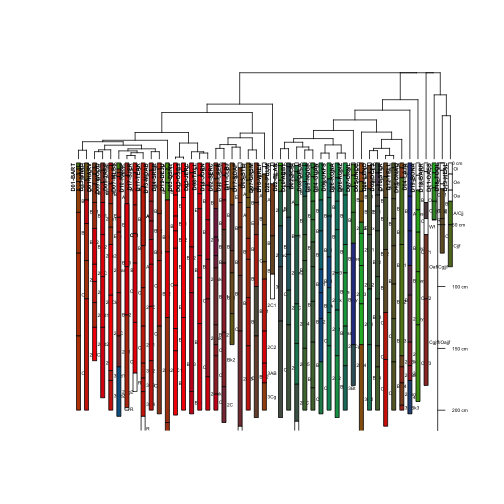
The clustering algorithm requires regularized data, so first we subset the data to records meeting the aqp package's quality standards, using the HzDepthLogicSubset() function.

# subset to meet quality threshold

S.sub <- HzDepthLogicSubset(S)

## dropping profiles with invalid depth logic, see `metadata(x)$removed.profiles`

# classify soil profiles

d <- NCSP(S.sub, vars=c('clayTotal',
                        'sandTotal', 
                        'siltTotal'), 
          k=0)

## Computing dissimilarity matrices from 33 profiles

##  [2 Mb]

## cache: 133 | slices: 300

# vizualize dissimilarity matrix via divisive hierarchical clustering

d.diana <- diana(d)



# Plot the resulting dendrogram

plotProfileDendrogram(S.sub, d.diana, scaling.factor = .6, 
                      y.offset = 2, width=0.25, cex.names=.4, 
                      name='horizonName.x', label='siteLabel', 
                      color='textureColor')

## dend.y.scale: 536

We have a dendrogram of the soil texture profiles.

To zoom in and vizualise more clearly, we need to make a plotting area large enough to contain the full plot with labels. To do so, we will open a PDF graphics device, generate the plot in that device, then close and save the device using dev.off(). It will also be a good idea to check your current working directory, and perhaps change that to where you want to save your PDFs.

# Check and set working directory as needed.

getwd()

## [1] "/Users/clunch/data"

# setwd("enter path to save PDF here")



# Open 'pdf' graphic device. Define file name and large dimensions

pdf(file="NEON_Soils_Texture_Color_Clusters.pdf", width=24, height=10)



# set plot margins and generate plot

par(mar=c(12,2,10,1), mfrow=c(1,1), xpd=NA)

plotProfileDendrogram(S.sub, d.diana, scaling.factor = .6, 
                      y.offset = 2, width=0.25, cex.names=.4, 
                      name='horizonName', label='siteLabel',
                      color='textureColor')

## dend.y.scale: 536

# Close and save the device

dev.off()

## quartz_off_screen 
##                 2

This plot is not shown on this tutorial webpage, but you can view and download an example of the PDF here.

Clustering by Nutrients

Rather than cluster based on physical properties, we can also cluster based on nutrient contents (nitrogen, carbon, and sulfur):

## Cluster as above, but for nutrient variables

d.nutrients <- NCSP(S.sub, 
                    vars=c('nitrogenTot',
                           'carbonTot', 
                           'sulfurTot'),
                    k=0)

## Computing dissimilarity matrices from 33 profiles [2 Mb]
## cache: 133 | slices: 300

# vizualize dissimilarity matrix via divisive hierarchical clustering

d.diana.nutrients <- diana(d.nutrients)

Let's make another PDF for our plot. However, this time it isn't as straightforward to plot the three nutrients of interest as 'rgb' colors, so we will make three separate plots for each nutrient:

# Open 'pdf' graphic device. Define file name and large dimensions

pdf(file="NEON_Soils_Nutrient_Clusters.pdf", width=24, height=14)



# Set plot margins

par(mar=c(8,2,5,1), mfrow=c(3,1), xpd=NA)



# Make plots for each nutrient of interest

plotProfileDendrogram(S.sub, d.diana.nutrients, scaling.factor = .6, 
                      y.offset = 2, width=0.25, name='horizonName', 
                      label='siteLabel', color='nitrogenTot',
                      col.label='Total Nitrogen (g/Kg)', 
                      col.legend.cex = 1.2, n.legend=6, 
                      col.palette=viridis::viridis(8))

## dend.y.scale: 558

plotProfileDendrogram(S.sub, d.diana.nutrients, scaling.factor = .6, 
                      y.offset = 2, width=0.25, name='horizonName', 
                      label='siteLabel', color='carbonTot',
                      col.label='Total Carbon (g/Kg)', 
                      col.legend.cex = 1.2, n.legend=6, 
                      col.palette=viridis::viridis(8))

## dend.y.scale: 558

plotProfileDendrogram(S.sub, d.diana.nutrients, scaling.factor = .6, 
                      y.offset = 2, width=0.25, name='horizonName', 
                      label='siteLabel', color='sulfurTot',
                      col.label='Total Sulfur (g/Kg)', 
                      col.legend.cex = 1.2, n.legend=6, 
                      col.palette=viridis::viridis(8))

## dend.y.scale: 558

# Close and save the device

dev.off()

## quartz_off_screen 
##                 2

This plot is not shown on this tutorial webpage, but you can view and download an example of the PDF here.