Introduction to NEON Fish Capture Data

This tutorial explores NEON fish capture data from sampling methods including electrofishing, gill netting, and fyke netting across NEON's lake and wadeable stream sites. NEON's fish data are stored across multiple interconnected tables that separately track individual fish measurements, bulk species counts, and details about sampling effort. Learning to properly join and summarize these tables is essential for calculating accurate abundance and diversity metrics.

Analysis of NEON fish data requires calculation of a fundamental metric: the total number of fish captured per species during a sampling event. This total capture count serves as the basis for calculating abundance, diversity indices, community composition, and detecting changes over time. The structure of DP1.20107.001 splits capture information across multiple tables, requiring users to perform an intermediate processing step in order to calculate total fish captures.

By the end of this tutorial, you will be able to download NEON fish count data, perform quality checks to ensure data integrity, join individual and bulk count tables appropriately, and summarize the results to generate the species-by-pass capture matrices that form the foundation of most fish community analyses.

1. Setup

Load R Packages

library(neonUtilities)

library(ggplot2)

library(dplyr)

library(tidyr)

Download NEON Fish Data

Download Fish electrofishing, gill netting, and fyke netting counts data using the loadByProduct() function in the neonUtilities package. Inputs needed to the function are:

• dpID: data product ID; Fish electrofishing, gill netting, and fyke netting counts = DP1.20107.001
• site: (vector of) 4-letter site codes; BLUE (stream site) & CRAM (lake site) in this tutorial
• package: basic or expanded; we'll download basic here
• check.size: should this function prompt the user with an estimated download size? Set to FALSE here for ease of processing as a script, but good to leave as default TRUE when downloading a dataset for the first time.
• startdate and enddate: we will work with 2024 data in this tutorial
• release: a particular data release, or current for the most recent release

Refer to the cheat sheet for the neonUtilities package for more details.

For more background on NEON data structures and use of the neonUtilities package, follow the Download and Explore NEON Data tutorial.

fshdat <- neonUtilities::loadByProduct(
  dpID="DP1.20107.001",
  site=c("BLUE", "CRAM"),
  package="basic",
  check.size = FALSE,
  startdate = "2024-01",
  enddate = "2024-12",
  release = 'RELEASE-2026')

NEON Data Citation

The use of NEON data should be cited according to our Data Policies & Citation Guidelines.

The data used in this tutorial were collected at the National Ecological Observatory Network's field sites.

• NEON (National Ecological Observatory Network). Fish electrofishing, gill netting, and fyke netting counts (DP1.20107.001), RELEASE-2026. https://doi.org/10.48443/s1e6-df79

2. Compiling the NEON Fish Data

The data are downloaded into a list of separate tables. Before working with the data, the tables are added to the R environment.

# View all tables in the list of downloaded fish data:

names(fshdat)

##  [1] "categoricalCodes_20107"     
##  [2] "citation_20107_RELEASE-2026"
##  [3] "fsh_bulkCount"              
##  [4] "fsh_fieldData"              
##  [5] "fsh_perFish"                
##  [6] "fsh_perPass"                
##  [7] "issueLog_20107"             
##  [8] "readme_20107"               
##  [9] "validation_20107"           
## [10] "variables_20107"

• The categoricalCodes file provides controlled lists used in the data

• The issueLog and readme have the same information that you will find on the data product landing page of the data portal.

• The fsh_fieldData table includes the date and time for all reach sampling efforts and will include an eventID value to indicate a unique bout of sampling in the 2026 release.

• The fsh_perPass table includes a record for each sampling pass conducted, and is linked to the field table through eventID and namedLocation.

• The fsh_perFish table includes records for each individually processed fish.

• The fsh_bulkCount table includes a count per species of fish captured after the specified number of individual fish are processed for the unique taxon or morphospecies.

• The validation file provides the rules that constrain data upon ingest into the NEON database.

• The variables file describes each field in the returned data tables.

Move the named items in the list to independent obejcts in the R environment:

list2env(fshdat, envir=.GlobalEnv)

The data about captured fish are in the fsh_perFish and fsh_bulkCount tables; we need to bring together the two data tables to get the full picture of all captures for each species.

Quality Verification

For bulk count data there should only be one bulk count record for each taxonID and pass. Before summarizing total captures across tables it is helpful to ensure bulk count records are present when expected.

bulkCount_count <- fsh_bulkCount %>% 
  select(eventID, boutEndDate,  passNumber, scientificName, taxonID, namedLocation, bulkFishCount) %>%
  group_by(eventID, boutEndDate, passNumber, namedLocation, scientificName, taxonID) %>%
  count()



unique(bulkCount_count$n)


## Number of bulk count records for each taxonID and pass: 1

The expected number of bulk count records exist, so we are able to proceed with processing.

Subset the data

First the bulk count data should be subset to only the necessary columns, to help keep the final summary output concise.

bulkCount_sub <- fsh_bulkCount %>% 
  select(eventID, passStartTime, passEndTime, boutEndDate,
         passNumber, namedLocation, barrierSubReach, 
         scientificName, taxonID, bulkFishCount)

Calculate the number of individual fish processed per pass

Before joining individual fish data with bulk count data to calculate total rates of capture, the total number of individual fish in the per fish table must be summarized for each pass. Per fish data is grouped by eventID, passNumber, namedLocation, barrierSubReach, and taxonID before tallying records for each taxon.

perFish_total <- fsh_perFish %>%
  select(eventID, passStartTime, passEndTime, boutEndDate, passNumber, 
         namedLocation, barrierSubReach, scientificName, taxonID) %>%
  group_by(eventID, passStartTime, passEndTime, boutEndDate, passNumber, 
         namedLocation, barrierSubReach, scientificName, taxonID) %>%
  count(name = 'individualFishCount')

Join individual and bulk count tables

Many analyses of NEON data will require the joining of two or more data tables that contain different sets of information. Details about which tables can be joined together and what variables should be used to link tables can be found in the "Table joining" section of the Quick Start Guide on each data product details page.

In this case, we can't make a simple join on the original tables, because the resolution of the two tables is different. The fsh_perFish table contains detailed information about individual fish captures, while the fsh_bulkCount table contains aggregate information about additional fish that were not processed individually and instead counted in bulk. Now that we have aggregated the fsh_perFish to a count per species, we can join to the fsh_bulkCount data.

fsh_all <- perFish_total %>%
  full_join(., bulkCount_sub, by=c('eventID', 'passStartTime', 'passEndTime', 
                                   'boutEndDate', 'passNumber', 
                                   'namedLocation', 'barrierSubReach', 
                                   'scientificName', 'taxonID'))

Calculate total captures

There are now two columns in the new fsh_all data frame that contain capture numbers for each unique pass - one with total number of fish in the fsh_perFish table, and one with total number of fish in the fsh_bulkCount table. These two values can be added to calculate the total number of fish captured per pass.

fsh_all <- fsh_all %>%  
  mutate(
    totalFishCount = rowSums(across(c(individualFishCount, bulkFishCount)), na.rm = TRUE))

The joined fsh_all table now contains the total number of fish captured per species for each pass, as well as the individual and bulk tallies for each species. The newly-calculated totalFishCount field will be used for all further community and population estimates.

Visualize results

Wadeable Streams

We can visualize abundance of each species for a particular site and event. In this tutorial, let's first look at the total number of captures for each species per pass at Blue River during the Spring of 2024.

# Subset summary data by eventID

blue_spring24 <- fsh_all %>%
  filter(eventID == "BLUE.2024.spring")


# Plot total captures by pass number and species

ggplot(blue_spring24, aes(x = scientificName, y = totalFishCount, fill = factor(passNumber))) +
  geom_bar(stat = "identity", position = "dodge") +
  coord_flip() +
  facet_wrap(. ~ namedLocation, scales = "free")+
  labs(title = "Fish Captures Across Sampling Passes: Blue River Spring 2024",
       x = "Species",
       y = "Total Fish Count",
       fill = "Pass Number") +
  theme_minimal() +
  theme(legend.position = "bottom")

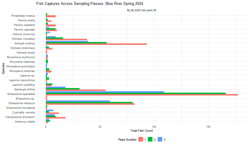
We can see that Blue River has a large diversity of species, as well as high capture rates at Fish Point 4. We can also see that the number of captures generally decreased between each consecutive pass, as is expected when depletion sampling.

Lakes

At lake sites, a total of five passes are recorded for fixed reaches, as opposed to the three passes at wadeable stream sites.

Information about fixed vs. random reaches is found in the fsh_fieldData table, and information about which sampling method is used for each pass is found in the fsh_perPass table. We can confirm that lake random reaches are only fished with a single electrofisher pass (Pass #1), one mini-fyke net pass (Pass #4), and one gill net pass (Pass #5), while lake fixed reaches are fished with all three electrofisher passes (Pass #1-3), as well as passes 4 and 5.

# Filter field data to desired eventID and view fixed vs. random reaches

fixedRandomReach <- fsh_fieldData %>% 
  filter(eventID=="CRAM.2024.fall") %>% 
  select(eventID, namedLocation, fixedRandomReach, samplingImpractical) %>% 
  arrange(namedLocation)



print(fixedRandomReach)

##          eventID              namedLocation
## 1 CRAM.2024.fall CRAM.AOS.riparian.point.03
## 2 CRAM.2024.fall CRAM.AOS.riparian.point.06
## 3 CRAM.2024.fall CRAM.AOS.riparian.point.07
## 4 CRAM.2024.fall CRAM.AOS.riparian.point.08
## 5 CRAM.2024.fall CRAM.AOS.riparian.point.09
## 6 CRAM.2024.fall CRAM.AOS.riparian.point.10
##   fixedRandomReach samplingImpractical
## 1            fixed                <NA>
## 2            fixed          logistical
## 3           random          logistical
## 4           random          logistical
## 5           random                <NA>
## 6            fixed          logistical

samplerType <- fsh_perPass %>% 
  filter(eventID== "CRAM.2024.fall") %>%
  select(eventID, namedLocation, passNumber, samplerType) %>% 
  arrange(namedLocation, passNumber)

        

print(samplerType)

##          eventID              namedLocation
## 1 CRAM.2024.fall CRAM.AOS.riparian.point.03
## 2 CRAM.2024.fall CRAM.AOS.riparian.point.03
## 3 CRAM.2024.fall CRAM.AOS.riparian.point.03
## 4 CRAM.2024.fall CRAM.AOS.riparian.point.03
## 5 CRAM.2024.fall CRAM.AOS.riparian.point.03
## 6 CRAM.2024.fall CRAM.AOS.riparian.point.09
## 7 CRAM.2024.fall CRAM.AOS.riparian.point.09
## 8 CRAM.2024.fall CRAM.AOS.riparian.point.09
##   passNumber   samplerType
## 1          1 electrofisher
## 2          2 electrofisher
## 3          3 electrofisher
## 4          4 mini-fyke net
## 5          5      gill net
## 6          1 electrofisher
## 7          4 mini-fyke net
## 8          5      gill net

Now let's take a look at the capture data from Crampton Lake during the Fall of 2024, which contains data from one fixed reach and one random reach.

# Subset summary data by eventID

cram_fall24 <- fsh_all %>%
  filter(eventID == "CRAM.2024.fall")


# Plot total captures by pass number and species

ggplot(cram_fall24, aes(x = scientificName, y = totalFishCount, fill = factor(passNumber))) +
  geom_bar(stat = "identity", position = "dodge") +
  coord_flip() +
  facet_wrap(. ~ namedLocation)+
  labs(title = "Fish Captures Across Sampling Passes: Crampton Lake Fall 2024",
       x = "Species",
       y = "Total Fish Count",
       fill = "Pass Number") +
  theme_minimal() +
  theme(legend.position = "bottom")

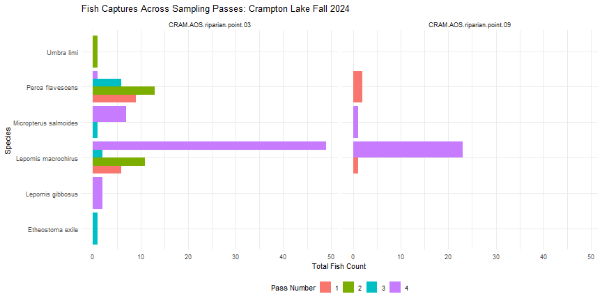In Fall 2024, it looks like no fish were captured using gill nets (Pass #5) at Crampton Lake.

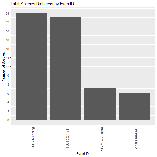
3. Visualizing Species Richness

Next, we can calculate species richness for each unique eventID, to examine the total number of species captured during each sampling bout.

Calculate richness for each eventID

Species richness represents the total number of fish species present within a habitat or ecological community. Species richness varies greatly across NEON sites, and can vary spatially within sites and also throughout time. We calculate richness by tallying the number of unique taxa recorded for each eventID.

richness_by_event <- fsh_all %>%
  select(eventID, scientificName) %>%
  group_by(eventID) %>%
  distinct(scientificName) %>%
  summarise(numSpecies = n()) %>%
  arrange(-numSpecies)

Now we can visualize the results.

ggplot(richness_by_event, aes(x = eventID, y = numSpecies)) +
        geom_bar(stat = "identity") +
        scale_x_discrete(limits = richness_by_event$eventID) +
        theme(axis.text.x = element_text(angle = 90)) +
        scale_y_continuous(breaks = seq(from = 0, to = 30, by = 2)) +
        labs(
          title = "Total Species Richness by EventID",
          x = "Event ID",
          y = "Number of Species"
        )